
Advantages of Adaptive PID Control System
Technical Article · TEC Controllers
A TEC controller needs a well-tuned PID loop to hold temperature. An adaptive PID controller finds its own loop settings, so you do not need to design and tune an external compensation network by hand.
Saves design time
No compensation network to design and tune by hand.
Saves PCB space
No external RP, CI, RD, and CD parts on the board.
Easy to use
No loop-tuning experience is needed to get a stable result.
Lowers cost
Reduces component, labor, and time costs.
What Is an Adaptive PID Control System?
PID stands for proportional, integral, and derivative. A PID controller compares the measured temperature with the set-point temperature. The difference is the error. The controller then combines three actions to decide how much current to send to the TEC:
| Term | What it reacts to | What it does in a TEC loop |
|---|---|---|
| P – Proportional | The present error | Gives a correction that is larger when the error is larger. |
| I – Integral | The error added up over time | Removes the small error that P alone leaves behind, so the object settles at the set point. |
| D – Derivative | How fast the error is changing | Acts early when the temperature moves fast. This reduces overshoot and oscillation. |
A standard PID controller uses fixed gains. Someone has to choose them. An adaptive PID controller has a self-learning function. It tests the actual load, calculates suitable gains by itself, and can repeat the test when the load or the ambient conditions change.
How a Manual Compensation Network Is Built
A TEC controller without adaptive PID needs an external compensation network to hold the object at the required temperature. The steps below show why each part of the network is needed.
Step 1Without feedback, temperature cannot be held
If the controller drives the TEC without measuring the result, nothing corrects the output. Heat load, ambient temperature, and TEC performance all change, so the object temperature drifts away from the set point.
Step 2Add feedback
A thermistor measures the object temperature and feeds it back to the input. The controller compares the measured temperature with the set point and generates an error signal. The P, I, and D functions then act on this error.
Add derivative action to stop oscillation
Feedback alone has a new problem: delay. Heat takes time to move from the TEC to the object and then to the thermistor. By the time the controller sees a change, the temperature has already moved further. If the gain is high, the controller over-corrects again and again, and the temperature oscillates.
The derivative (D) term responds to how fast the temperature error is changing. When the temperature moves quickly toward the set point, the D term reduces the correction. This helps suppress overshoot and oscillation.
Step 4Add integral action to remove the remaining error
With P and D only, a small steady error usually remains. The integral (I) part adds up this error over time and slowly increases the correction until the error reaches zero. The object then settles at the set point with high accuracy. Too much integral action makes the response slow or causes overshoot, so it must be balanced with P and D.
Why manual tuning takes so long: RP, CI, RD, and CD interact. After RP is set to its best value, any change to CI, RD, or CD shifts the best RP value again. An engineer who tunes a loop for the first time may need several weeks or more. An experienced engineer may still need several days to a week to find settings that work well for a given load.
How Adaptive PID Control Works
Adaptive PID control puts the function of the compensation network into a single chip. The chip runs a self-learning test on the actual load and environment, then calculates a set of PID gains. This replaces the external network. The learning process takes only a few minutes. If the load or the environment changes, the controller simply learns again.
Closed-loop self-learning
Adaptive tuning methods are usually grouped into open-loop, closed-loop, and relay methods. This article covers the closed-loop method.
In the closed-loop method, the loop gain is adjusted until the loop oscillates as a steady sine wave that is not saturated. The gain at this point is KC, and the period of the oscillation is T. The PID gains are then calculated from KC and T:
These are the classic Ziegler–Nichols closed-loop tuning rules. They give an integral time of T/2 and a derivative time of T/8.
Advantages of Built-In Adaptive PID Control
Analog Technologies has built adaptive PID control into its TEC controllers. The TEC28V15ADAPID is a TEC controller with built-in adaptive PID control. It replaces the external compensation network, and it can learn again when the load or the ambient temperature changes.
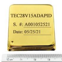
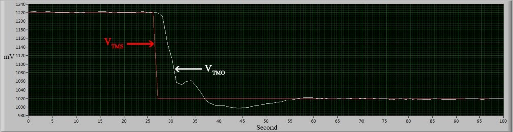
Figure 6 compares two waveforms. VTMO is from the TEC28V15AD, which uses a manually tuned compensation network. VTMS is from the TEC28V15ADAPID, which uses its built-in adaptive PID control.
| Item | Manual compensation network | Built-in adaptive PID |
|---|---|---|
| Setup time | Several days to several weeks, depending on experience | A self-learning run of a few minutes |
| External parts | RP, CI, RD, and CD on the PCB | None for loop compensation |
| Skill needed | Loop-tuning experience | Switch to “Learn”, then to “PID” |
| Load or ambient change | Re-tune the parts by hand | Run the learning again |
Because setup is fast and does not depend on tuning skill, a TEC controller with built-in adaptive PID control fits a wider range of projects.