
TEC Controller: How It Works and How to Choose the Right One
Engineering White Paper · AWP-TECC-02 · Rev 2.8
TEC Controller: What It Is and How to Choose One
A practical OEM guide to TEC controller architecture, stability, output-stage topologies, and a six-step selection methodology that ends at a specific ATI part number.
Current and voltage are separate problems
The 1.5–2× current factor does not apply to voltage. Size each against its own constraint.
Topology sets the ceiling
Linear, PWM, or hybrid determines efficiency, ripple, EMI, and whether precision-grade stability is reachable.
Stability is measured at the sensor
±0.001 °C describes the feedback point under defined lab conditions, not the temperature at the load.
Validate before layout
Confirm the selection on the matched evaluation board against the real TEC, sensor, and thermal load.
Summary — Choosing a TEC Controller
A TEC controller is a closed-loop thermal servo: it reads a temperature sensor (typically an NTC thermistor), compares the measurement against a programmable setpoint, computes a PID correction, and drives regulated bidirectional current into a thermoelectric (Peltier) cooler to hold the load at the target temperature.
This guide covers what a TEC controller is at engineering depth — closed-loop architecture, output-stage topologies, compensation theory, stability and noise specifications, and the protection circuitry that makes a module-level controller different from a TEC driver IC — and then turns that understanding into a six-step selection methodology that takes a designer from the application’s thermal load, setpoint, ambient envelope, supply rail, and EMI environment to a specific ATI TEC controller family, precision grade, suffix variant, and evaluation board.
ATI’s precision-analog families (TEC14M, TECA1, TEC5V4A, TEC5V6A) and high-current series (TEC18V15A, TEC24V10A, TEC24V15A) are described in full, and five worked application examples — laser-diode wavelength stabilization, PCR / high-current instrumentation, outdoor kiosk cooling, miniaturized photonic sensors, and LIDAR receivers — each produce a starting ATI controller part number for engineering evaluation.
Six-step checklist
- Characterize the cold-side thermal load Q_load (active dissipation plus passive heat gain).
- Define the target setpoint, worst-case ambient temperature, and design priority (precision, size, autonomous operation, low EMI).
- Determine the TEC module operating-point current I_TEC and voltage V_TEC from the datasheet at the actual operating point — TEC module sizing is covered in companion paper AWP-TECC-03.
- Match the controller current and voltage capability. Rated I_max ≥ I_TEC × 1.5–2× current headroom (a starting guideline for many OEM designs; final headroom depends on TEC derating, transient requirements, and current-limit setting); output voltage and supply-rail capability must cover V_TEC plus dropout at worst-case hot ambient.
- Choose the output-stage topology and precision grade. Linear, PWM, or hybrid; D, DA, or DAH — appropriate to the application’s EMI environment and stability target.
- Validate the selection on the matched evaluation board against the actual TEC, sensor, and thermal load.
Read this paper if…
You need to choose the TEC controller for an OEM thermal-control product: current, voltage, supply rail, output-stage topology, precision grade, suffix variant, and evaluation board. If instead you need to design the thermal stack — TEC module sizing, heat sink, Q_hot, sensor placement, mounting, condensation control, and validation — the companion paper AWP-TECC-03 (How to Design a TEC Cooling System) is the right starting point.
Critical caveats. (a) Current headroom and voltage headroom are separate engineering problems — the 1.5–2× current factor does not apply to voltage. (b) The controller’s programmed current limit must protect the TEC at its safe maximum current at the operating hot-side temperature, independent of the controller’s rating headroom. (c) Stability figures quoted in controller datasheets (e.g., ±0.001 °C at DAH grade) are measured at the sensor under defined laboratory conditions; the achievable temperature at the controlled object depends on sensor placement, mounting, heat-sink stability, airflow, and ambient drift, addressed in AWP-TECC-03. (d) Sub-10 mK stability at the load is a system-level outcome — controller choice is necessary but not sufficient.
Why ATI for OEM TEC controllers
ATI is a supplier of matched TEC controllers, TEC modules, precision thermistors, and evaluation boards, supporting OEM customers across North America, Europe, and Asia. ATI supports OEM programs with lifecycle communication, replacement guidance, and applications-engineering support where available; for any specific part-level migration questions, contact ATI sales. The hybrid topology (U.S. Patent 6,486,643 B2) is the basis for the precision controller line and delivers high efficiency together with low output ripple in a single module.
In a hurry? Jump to §4 Selection Methodology for the six steps, §7 ATI Product Families for the master comparison table, or §8 Application Examples to see worked solutions in your application area.
| Topic | Canonical paper |
|---|---|
| Beginner / visual explanation of a TEC controller | AWP-TECC-01 — What Is a TEC Controller? (Visual Engineering Guide) |
| TEC controller — what it is and how to choose one (this paper) | AWP-TECC-02 (this paper) |
| TEC cooling system design — TEC module sizing, heat-sink sizing, sensor placement, mounting, validation | AWP-TECC-03 — How to Design a TEC Cooling System |
| Thermoelectric cooler fundamentals — what a TEC module is | AWP-TECM-01 — What Is a Thermoelectric Cooler? |
| Multi-TEC arrays and cascade systems for high cooling loads | AWP-TECM-03 — Multi-TEC Thermal System Design |
Part I — Foundations
What a TEC controller is, what it is not, and the specifications that drive every later decision.
1. Why TEC Controller Selection Matters
Selecting a TEC controller is one of the highest-leverage decisions in a thermal-control design. The controller sets the achievable temperature stability, the efficiency of the thermal loop, the electromagnetic signature of the product, the cost of the bill of materials around the output stage, and the time to a working prototype. It strongly influences the heat-sink size as well (through output-stage efficiency and the resulting Q_hot), though the dominant heat-sink driver is the TEC, the application thermal load, and the worst-case ambient. Every other component — the TEC module, the temperature sensor, the heat sink, the power supply — interacts with the controller selected for the design.
Common consequences of a poor controller match: insufficient current headroom causes the loop to saturate at worst-case ambient; insufficient voltage prevents the loop from reaching the ΔT a precision application requires; the wrong topology injects switching noise into nearby sensitive analog circuits; an inappropriate precision grade passes the bench test but fails production temperature-cycle qualification. None of these failures are catastrophic in isolation, but each consumes weeks of redesign effort and pushes a product launch into the next quarter.
This guide is a structured framework. It assumes the engineer has already established that a closed-loop TEC controller is the right architecture for the application; what the engineer needs next is a path from the thermal-load requirement to a specific orderable part number. The guide walks that path in six steps, compares the three controller topologies (PWM, linear, and ATI’s hybrid), explains what temperature stability specifications actually mean in practice, and finishes with a side-by-side comparison of every ATI TEC controller product family. The objective is a controller decision the engineer can defend in a design review.
What is a TEC controller?
A TEC controller is a closed-loop electronic module that drives a thermoelectric cooler (Peltier element) to hold a thermal load at a programmable target temperature. It reads a temperature sensor (NTC thermistor, RTD, or IC sensor), compares the measurement to a setpoint voltage, computes a PID correction signal, and delivers regulated bidirectional current to the TEC — heating or cooling automatically as needed to reach and hold the setpoint. Stability of ±0.001 °C is achievable with precision-grade controllers under defined test conditions (load-matched compensation, precision thermistor, stable ambient). Typical applications include laser-diode wavelength stabilization, photodetector and APD cooling, diagnostic and laboratory instrumentation, optical spectrum analyzers, and CCD/CMOS imager cooling.
Controller vs. driver vs. discrete op-amp loop
Engineers face three options when implementing thermoelectric temperature control. A closed-loop TEC controller module is a self-contained integrated assembly — it reads the sensor, runs the loop, and drives the TEC with no host software required for the analog-compensation families. A TEC driver IC is an open-loop building block: it sources a commanded current but does not close the temperature loop — the host MCU or FPGA must measure the sensor, run PID firmware, and command the driver. A discrete op-amp loop builds the equivalent function from individual op-amps, resistors, capacitors, and a power stage on the OEM PCB.
The trade-off across the three is integrated closed-loop control versus board space versus engineering effort: a controller module supports initial closed-loop validation quickly on an evaluation board against the actual TEC and load; a driver requires the OEM to write and debug firmware against the thermal model; a discrete loop requires extensive analog design and iteration. For OEM production where temperature stability matters and time-to-market is constrained, a dedicated TEC controller module removes much of the analog-loop design risk.
Scope of this guide
This paper covers TEC controllers for OEM thermal-control products with cooling-load requirements from 0.5 W to approximately 60 W per controller channel. Loads above this range are typically served by paralleled controllers or multi-TEC arrays — outside the scope of this paper but covered in the companion paper AWP-TECM-03: Multi-TEC Thermal System Design. System-level design — sizing the TEC module against the heat load, sizing the heat sink, sensor placement for low thermal resistance, mounting the TEC between load and heat sink, and validating the complete assembly — is treated in detail in AWP-TECC-03. This guide focuses on the controller itself.
Who this guide is for
The primary reader is the OEM design engineer selecting and integrating a TEC controller: photonics and laser-diode designers, medical and diagnostic instrument engineers, imaging-system designers, LIDAR receiver designers, and the technical purchasing managers who specify the bill of materials. The guide assumes working knowledge of analog electronics, basic closed-loop control theory, and the Peltier effect. Readers new to thermoelectric cooling should consult AWP-TECC-01: What Is a TEC Controller? (visual introduction) and AWP-TECM-01: What Is a Thermoelectric Cooler? (TEC module fundamentals) before proceeding here.
Quick-reference starting point
If the application’s cooling load and approximate ΔT are already known, the table below identifies a starting family. This table is a first-pass screening tool only — final controller selection must be based on the TEC module’s operating-point I_TEC and V_TEC read from the datasheet performance curves, not on Q_load alone. Work through the six-step methodology in §4 before locking the decision.
| Application Q_load | Typical ΔT | PCB constraint | Starting family |
|---|---|---|---|
| ≤ 1 W | ≤ 60 °C | Severely constrained, SMT | TEC14M |
| 1–4 W | ≤ 50 °C | Moderate, DIP acceptable | TECA1 or TEC5V4A |
| 4–10 W | ≤ 40 °C | Moderate, DIP acceptable | TEC5V6A |
| 10–50 W | ≤ 30 °C | Relaxed | TEC18V15A, TEC24V10A, or TEC24V15A |
| 10–60 W (enclosure) | Any | Enclosure cooling with fans | ATFC106D |
Note on the load-vs-ΔT trade-off: the table lists the application thermal load Q_load (sum of device dissipation, conduction, convection, and radiation at the cold side); the TEC module must provide Q_c ≥ Q_load at the operating ΔT. Higher loads require proportionally more electrical input to pump the heat (COP falls with both load and ΔT), so practical OEM designs at higher Q_load are normally specified at lower ΔT to keep input power, heat-sink size, and Joule self-heating manageable. Smaller loads can comfortably be designed at higher ΔT because the absolute power penalty is small. Applications that exceed this typical envelope — deep cooling at high Q_load — generally require multi-stage TECs or multi-module arrays. The table assumes a single-stage TEC and an adequately sized heat sink at the assumed worst-case ambient; the 60 W upper bound applies primarily to the enclosure-cooling row using ATFC106D.
Multi-stage sizing note: for cascade TEC stacks, the hot side of each upper stage becomes the cold-side load for the stage below it (Q_c,lower = Q_c,upper + P_electrical,upper). Each successive lower stage therefore sees a larger thermal load and draws proportionally more current, which compounds the controller and heat-sink sizing requirements. Multi-stage stacks generally require the high-current series (TEC18V15A, TEC24V10A, or TEC24V15A), and the heat sink must be sized for the cumulative Q_hot at the bottom-stage outer face.
Not sure where your application fits?
ATI applications engineering provides design review and starting-family recommendations for qualified OEM TEC controller, TEC module, and thermal-system projects. Send a short specification — cold-side thermal load Q_load, target temperature and worst-case ambient range, TEC module part number (if selected), available supply voltage, and any heat-sink or footprint constraints — and an applications engineer can review and recommend a starting family. Contact details and the full selection-support form are in §10.
Recommended starting family by application — quick answer
A compact lookup keyed by application type rather than load. For the load-and-ΔT view see the quick-reference table above; for the full methodology see §4; for worked examples in each application see §8.
| Application | Starting family | Example part number |
|---|---|---|
| Miniature photonics / SMT sensors | TEC14M | TEC14M5V3R5AS |
| Laser-diode cooling (1–3 W) | TECA1 or TEC5V4A (-LD variants) | TECA1-5V-5V-DAH or TEC5V4A-DAH-LD |
| Mid-power 5 V precision (4–10 W) | TEC5V6A (hybrid) | TEC5V6A-DAH (-LD for laser) |
| PCR / high-current instrumentation (10–50 W) | High-current series | TEC18V15A, TEC24V10A, or TEC24V15A |
| Kiosk / outdoor cabinet cooling (20–60 W) | ATFC (window mode + fan PWM) | ATFC106D |
| LIDAR receiver / APD cooling | TEC5V6A or high-current series | TEC5V6A-DAH or TEC24V10A |
| AI accelerator / GPU hotspot spreading | High-current series | TEC18V15A, TEC24V10A, or TEC24V15A |
Starting family only — verify before ordering. This table is a first-pass filter. Final part-number selection must verify TEC operating current, TEC operating voltage, controller output voltage and current margin, system supply rail, heat-sink thermal resistance, and worst-case ambient derating. Skipping the methodology in §4 is a common cause of field saturation and redesign in OEM products.
ATI services for OEM TEC system development
Applications engineering review for qualified OEM projects: ATI applications engineering can review TEC controller, TEC module, and thermal-system selection questions for qualified OEM applications. Send a short application specification to sales@analogtechnologies.com and an applications engineer can review the inputs and recommend a starting family, evaluation board, and matched TEC module.
Custom engineering for special and high-volume applications: beyond the standard catalog, ATI takes on TEC-related engineering projects — customized TEC modules (non-standard form factors, footprints, ΔT ranges, current ratings), customized TEC controllers (non-standard supply rails, footprint or pinout adaptations, suffix combinations, OEM-specific firmware configuration on the high-current series), and complete custom TEC assemblies and systems (matched controller + TEC + heat sink + sensor delivered as a tested subassembly). These projects are subject to engineering review, intended for qualified OEM volume programs or special applications, and typically require NRE and MOQ commitments with lead time depending on scope.
What are the most common TEC cooling system failure modes after correct component selection?
In OEM TEC cooling systems where the catalog components are reasonable for the application, the failure modes that show up in the field most often are not component-choice failures — they are system-design and assembly failures. The recurring ones are:
- Undersized heat sinks — using the TEC absolute-maximum hot-side rating in place of the temperature that still allows pumping Q_load at the required ΔT.
- Insufficient controller voltage headroom at deep ΔT and worst-case hot ambient (V_TEC rises with T_hot, and V_PS − V_dropout must still cover it).
- Thermistor placed on the TEC ceramic instead of the cold plate, or far enough from the controlled object that a thermal gradient appears between sensor and load.
- Excessive TIM thickness on the hot- and cold-side interfaces — more grease is not better; fill the voids and squeeze the rest out.
- Uneven mechanical compression that bows a thin cold plate and creates a center air gap.
- Condensation when the cold-side setpoint drops below the local dew point without sealing or dry-gas purge.
- Inadequate worst-case validation — passing at design ambient and failing at the upper ambient bound the product will actually see in service.
2. How a TEC Controller Works — Essentials
A closed-loop TEC controller samples the temperature of the load, compares the reading to a programmable setpoint, and adjusts the current through a Peltier element until the error converges. The loop runs continuously inside the controller; no host firmware is required for the closed-loop temperature regulation function once the controller is configured, although system firmware may still monitor, configure, or supervise the thermal subsystem depending on product architecture.
The amount of configuration required differs by family. The precision-analog families (TEC14M, TECA1, TEC5V4A, TEC5V6A) are largely standalone analog controllers — the setpoint, compensation network, and current/voltage limits are set with external components or pots, after which the loop runs without host involvement. The high-current series (TEC18V15A, TEC24V10A, TEC24V15A) is firmware-managed and exposes digital configuration of PID and Auto-PID parameters, current and voltage limits, and protection thresholds — once configured, the loop also runs without host involvement, but the initial setup and any field updates use the digital interface. The ATFC106D is a digital window-mode enclosure-cooling controller with its own setup model.
Five functional blocks
- Temperature sensor (NTC thermistor, platinum RTD, or IC sensor) bonded to the load.
- Error amplifier that subtracts sensor voltage from setpoint voltage.
- Compensation network (PID, with R-C components setting proportional gain, integral action, and derivative damping). Covered in §5b.
- Power output stage that converts the compensated signal to regulated bidirectional TEC current. Topology choices are covered in §3.
- Protection and monitoring including current limit, voltage clamp, thermal shutdown, and diagnostic outputs.
What is the difference between a TEC controller and a TEC driver?
The closed-loop architecture distinguishes a TEC controller from a TEC driver. A driver delivers commanded current without temperature feedback, leaving the host system to close the loop in firmware. A controller closes the loop in its own analog or digital domain. For OEM applications where temperature stability is the deliverable, the controller is generally the appropriate choice because it integrates sensor feedback, compensation, protection, and TEC power-stage drive on a single module, reducing host firmware and loop-design burden.
Heating and cooling direction control
A Peltier element pumps heat in the direction of current flow. Reversing the current reverses the direction of heat pumping — the same face that was absorbing heat now rejects it. Bidirectional TEC controllers exploit this through an H-bridge output stage, in which four switching elements arrange to connect either polarity of the supply rail across the TEC terminals. Unidirectional controllers — useful in cooling-only or heating-only applications — use a simpler single-polarity output stage; this guide focuses on the bidirectional case that dominates precision OEM products.
When the loop calls for cooling (load above setpoint), the H-bridge routes current in the polarity that makes the load-side TEC face absorb heat. When the loop calls for heating (load below setpoint), the H-bridge reverses polarity and the same face now rejects heat. The transition is automatic, continuous, and managed entirely inside the controller — no external mode switch, no host firmware command, no relay required for TEC polarity reversal inside the control loop. The final product may still require fuses, disconnects, interlocks, or safety shutdowns dictated by its end-application and applicable safety standards.
Bidirectional drive matters when the application alternates between modes during normal operation: a laser-diode wavelength-stabilization loop that must cool in summer and heat in winter to hold the same wavelength; a PCR thermal cycler slewing between 4 °C and 95 °C; a refrigerated kiosk that cools by day and gently heats overnight to prevent condensation. Unidirectional controllers exist for applications that only ever cool or only ever heat, and they cost less, but bidirectional is the common default for precision OEM products that must both heat and cool around a setpoint.
In ATI’s bidirectional continuous-current TEC controllers — the precision-analog families and the high-current series, all of which use ATI’s hybrid topology — the controller’s closed-loop PID determines which polarity is needed and reverses the current direction through the Peltier element to switch between cooling and heating automatically. (The ATFC106D operates differently — it is a digital window-mode controller for enclosure-cooling applications that switches the TEC on and off within a temperature window rather than running closed-loop bidirectional drive; see §7 for its application envelope.)
Key specifications that drive selection
Four parameters dominate datasheets and selection decisions. The remainder of this guide returns to each in detail.
- Maximum output current (I_max). Highest TEC current the controller can deliver continuously. Must exceed the TEC’s operating-point current — §4.
- Maximum output voltage (V_max). Peak voltage across the TEC terminals. Sets achievable ΔT — §4.
- Temperature stability. Peak-to-peak variation of the regulated temperature at steady state over a stated window. “Regulated temperature” means the temperature at the sensor connected to the controller’s feedback input. The temperature at the load (e.g., laser-diode junction) will differ due to thermal gradients across the package, sensor placement, and mounting variability. Distinct from accuracy and resolution — §5.
- Efficiency. Power delivered to the TEC divided by power drawn from the supply. Topology-dependent — §3.
Part II — Controller Topologies
How the output stage is built, and what that choice costs in efficiency, ripple, EMI, and board area.
3. PWM vs. Linear vs. Hybrid TEC Controllers
The power output stage of a TEC controller can be built three ways. Each carries a characteristic efficiency, ripple, EMI, and BOM-cost signature. Most engineers inherit this choice from a legacy block diagram without recognizing that it largely determines whether the system can reach precision-grade stability — and whether the controller itself runs cool or requires significant thermal management of the controller package.
Which TEC controller topology should I choose?
For most precision OEM applications — laser-diode cooling, photonics, medical instruments — a hybrid topology that combines a switch-mode stage with a linear post-regulation stage delivers the best balance: efficiency close to pure switch-mode, output ripple substantially lower than pure PWM (the linear post-regulator scrubs the residual switching edges from the switch-mode leg, with the absolute level depending on operating current and the specific implementation), and component count comparable to or below either. Pure linear topologies remain appropriate for ultra-low-EMI benchtop applications; pure PWM can be appropriate where switching ripple and EMI are already managed at the system level and high efficiency is the dominant constraint.
Linear-mode controllers
A linear TEC controller regulates output current through an analog pass element — typically a power MOSFET or bipolar transistor operating in its linear (non-saturated) region. The pass element acts as a continuously variable resistor between the supply rail and the TEC, dissipating the difference between supply voltage and TEC voltage as heat in the transistor itself.
Strengths: zero switching ripple, the simplest possible architecture, no LC filter required, no switching EMI from the output stage itself — a particular advantage in audio or RF-sensitive systems where switching harmonics would otherwise need to be designed out. System-level EMC still depends on wiring, sensor-lead routing, grounding, supply-noise paths, and load-current returns, all of which remain the integrator’s responsibility.
Limitations: efficiency is bounded by the ratio of TEC voltage to supply voltage, typically in the 20–40% range. The remaining 60–80% of input power is dissipated as heat in the pass element, which must itself be cooled, adding size, weight, and BOM cost. At full output power, the controller runs hot enough to require thermal-management attention in its own right.
Best fit: low-power applications where ripple specifications tolerate no switching artifacts, ultra-low-EMI environments such as precision metrology and high-resolution analog instrumentation, and benchtop instruments where size and weight are not constraints.
PWM (switch-mode) controllers
A PWM TEC controller chops the supply voltage on and off at a high switching frequency — typically 100 kHz to 1 MHz — and uses an LC filter to smooth the chopped waveform into regulated DC current for the TEC. The duty cycle sets the average current; the inductor and capacitor remove the switching ripple.
Strengths: efficiency in the 85–93% range, no continuous-conduction loss in the pass element (only switching losses in the FETs), small magnetics, low controller self-heating, compact form factor at high output power.
Limitations: output ripple — representative range 1–5% of average current for typical TEC controller PWM designs, but the actual value depends on PWM frequency, output LC filter (if any), TEC impedance, layout, and control method — contributes I²R Joule heating in the TEC without contributing to Peltier cooling, reducing effective Q_c. Switching edges radiate electromagnetic interference that can couple into nearby sensitive analog circuits such as laser-diode drivers, photodiode front ends, and precision ADCs. The LC filter adds component count, PCB area, and inductor cost.
Best fit: higher-power applications (above ~5 W) where efficiency is a priority, space-constrained OEM products, and systems that already accept switching power supplies elsewhere so the EMI environment is established.
Hybrid topology — ATI’s patented approach
A hybrid topology places one switch-mode leg and one linear leg in the H-bridge output. The switching leg delivers high efficiency; the linear leg acts as a low-noise post-regulator that scrubs the residual ripple from the switching leg before it reaches the TEC. The combination targets high efficiency and low ripple in the same module, without the large external LC output filter normally associated with pure dual-PWM TEC drive — final system EMC still depends on layout, grounding, shielding, cable treatment, and any required product-level filtering.
Strengths: approximately 90% efficiency at the standard test point (V_out = ½ V_PS, I_out = ½ rated I_max) — about 37% less output-stage power loss than a reference dual-PWM controller architecture at the same operating point. These figures are from an ATI internal 5 V, 3 A reference-design characterization — not a competitor benchmark or universal device-level guarantee; actual results depend on operating point, layout, and integration. Output ripple is lower than pure-PWM topologies operated without external LC filtering, under similar operating conditions; for specific measured ripple, see the family datasheet. Component count and PCB area are also reduced compared to a reference dual-PWM bridge of equivalent capability — approximately 27% lower component cost and 33% smaller PCB area in ATI’s reference implementation. ATI’s topology is based on U.S. Patent 6,486,643 B2 (G. Liu, 2002), assigned to Analog Technologies, Inc.
Limitations: the linear leg still dissipates some power and runs warmer than a pure-PWM controller of equivalent output; the topology is not optimal at very low output currents where the linear stage’s dropout becomes a significant fraction of the TEC voltage.
Best fit: the majority of OEM products that require both efficiency (battery life, modest controller cooling) and precision (laser-diode wavelength stability, photonics, low-noise medical sensors). The hybrid topology is the architectural basis for the ATI continuous-current TEC controller families covered in this guide — the precision-analog families and the high-current series alike. The high-current series differs from the precision-analog families in supply rail, current capability, and the addition of firmware-managed digital configuration (Auto-PID, programmable protections, digitally-set PID and limit parameters) — not in output-stage topology. The ATFC106D is a separate product category: a window-mode enclosure-cooling controller that switches the TEC on and off across a temperature window rather than running closed-loop continuous bidirectional drive.
Hybrid topology vs a reference dual-PWM architecture: quantified benefits
Conventional bidirectional TEC controllers use two PWM output stages in an H-bridge configuration to support cooling and heating. The ATI hybrid topology replaces one of those PWM stages with a low-dissipation linear post-regulator, while keeping the same control electronics. The PCB area, component cost, and output-stage efficiency benefits are quantified in the table below using a reference implementation example calculated from ATI engineering values for a typical 5 V, 3 A TEC controller — representative of the precision-analog families — not measured side-by-side against a specific competitor product. The values are normalized: 1 area unit and 1 cost unit each represent the footprint and BOM contribution of the controller’s PWM output stage in this reference design.
| Metric | ATI hybrid | Conventional dual-PWM | Representative reduction |
|---|---|---|---|
| PCB area: control + linear stage | 1 area unit | 1 area unit (control only) | — |
| PCB area: PWM output stage(s) | 1 area unit (×1 PWM) | 2 area units (×2 PWM) | — |
| Total PCB area | 2 area units | 3 area units | ~33% smaller |
| Component cost: all controller components | 4 cost units total | 4 + 1.5 cost units (extra PWM) | — |
| Total component cost | 4 cost units | 5.5 cost units | ~27% less |
| Power loss: PWM stage(s) | 8% (×1 stage) | 16% (×2 stages × 8%) | — |
| Power loss: linear stage | 2% | — | — |
| Total output-stage power loss | ~10% | ~16% | ~37% less loss |
Topology comparison summary
| Metric | Pure linear | Pure PWM | ATI hybrid topology |
|---|---|---|---|
| Efficiency (typical) | 20–40% | 85–93% | >90% at standard test point |
| Output ripple | <0.05% | 1–5% (typically requires output filtering for precision use) | Low without external filter; see family datasheet for measured value |
| Switching EMI | None | Radiated + conducted | Linear post-regulator attenuates switching ripple at the TEC output; package design varies (shielded module on DIP families, board-level layout on SMT TEC14M). System-level EMC still requires layout, grounding, and external filtering design. |
| Component count (output stage) | Lowest | Moderate (FETs + L + C) | Lower than dual-PWM bridges |
| Controller self-heating | Significant | Low | Moderate |
| Best fit | Linear-only benchtop, ultra-low-EMI | High-power, EMI-tolerant | Common starting point for precision OEM designs |
Standard ATI efficiency test point: V_out = ½ V_PS, I_out = ½ rated I_max. This is the operating-point convention used across ATI’s hybrid families; efficiency figures measured at different operating points (very low or very high load) will differ. Engineers comparing efficiency across vendors should ensure the same test point.
Why this matters for OEM design
For OEM products where the controller sits next to a laser driver, photodetector front end, or precision ADC, the hybrid topology reduces the LC-filter design effort and the EMI mitigation work that pure-PWM controllers typically require. ATI uses the hybrid topology across the continuous-current TEC controller families covered in this guide — the precision-analog families (TEC14M, TECA1, TEC5V4A, TEC5V6A) that serve loads up to roughly 6 A on a 5 V supply, and the high-current series (TEC18V15A, TEC24V10A, TEC24V15A) that serves loads up to 15 A on 6–24 V rails. Across both ranges the engineering goal is the same: precision drive without the LC-filter and EMI overhead of a reference dual-PWM architecture.
Part III — Selection Methodology
Six steps from a thermal-load specification to a starting ATI part number, and what the stability numbers actually mean.
4. Six-Step TEC Controller Selection Methodology
Selecting a TEC controller for an OEM product is a structured calculation. The thermal load, target temperature, worst-case ambient, available supply rail, TEC module, and heat sink are not independent choices — they form a coupled system that must be sized together. This section walks through the controller-selection decision in six steps; Steps 1, 3, and 6 (thermal load, TEC module sizing, heat-sink sizing) are summarized here because they form the inputs to controller selection, and are covered in full detail in companion paper AWP-TECC-03. Steps 2, 4, 4b, and 5 are the heart of the controller decision and are detailed here.
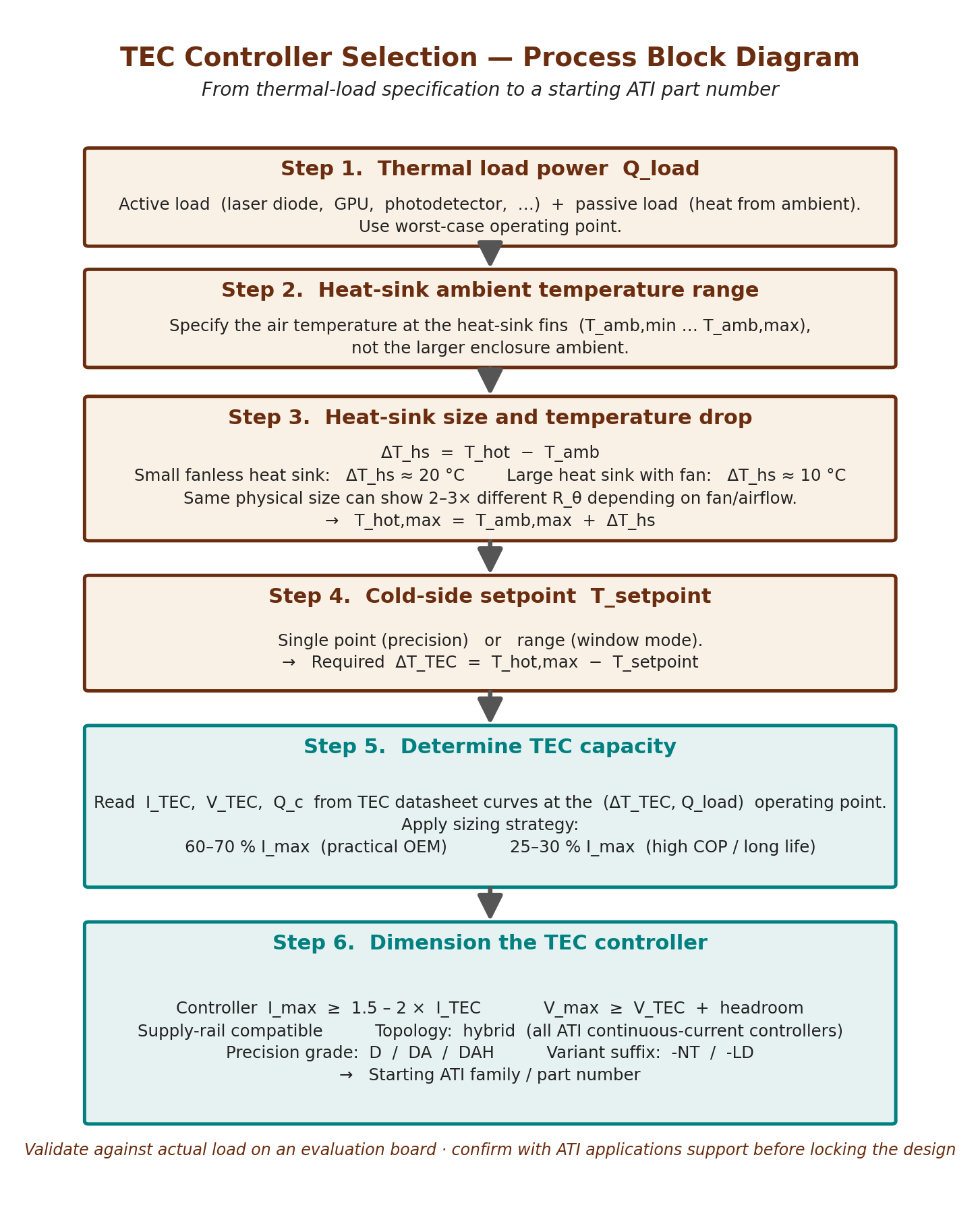
Sizing a TEC controller is a six-step calculation. Each step constrains the controller selection more tightly than the last. By the end the engineer has a specific product family — and, with the additional refinement in §5b on precision grade and variant suffix, a specific part number.
Step 1 — Define the cold-side thermal load Q_load (brief)
Q_load = Q_active + Q_passive
This is the total heat the TEC must move from the cold side, summed over active sources (device dissipation: laser-diode electrical-to-optical inefficiency, photodetector bias, CCD readout, sensor electronics) and passive sources (heat flowing into the cold object from warmer surroundings via conduction through wires and mounting hardware, convection, and radiation; significant when the setpoint is well below ambient).
Typical values: fiber-coupled telecom laser diode 0.5–2 W; free-space DFB 1–5 W; PCR well during ramp 10–30 W; OCXO oven 1–3 W; cooled CMOS image sensor at deep ΔT 3–15 W; refrigerated kiosk display compartment 20–60 W.
For full Q_load decomposition (active/passive separation, calculated vs. measured passive load, optical-absorber and solar-flux cases, and the worst-case operating-point convention), see AWP-TECC-03, §3.
Step 2 — Define temperature requirements
Three temperatures matter, not one.
- Target object temperature (setpoint). Fixed value (a laser at 25.000 °C) or programmable range (a thermal cycler running 4 °C to 95 °C). The range determines whether a fixed-range variant suffices or whether the engineer needs the wider configurability of a -NT variant — §5b.
- Worst-case ambient temperature at the heat sink. Not room temperature — the worst-case temperature the heat sink will actually see in the field. Account for sunlit enclosure walls, dust accumulation, adjacent equipment, and seasonal extremes. A thermal-management design that closes at 25 °C lab ambient may fail at 50 °C in a hot environment.
- Required ΔT across the TEC. Defined as T_hot_side − T_cold_side, where T_cold_side is the object temperature and T_hot_side is the heat-sink-side TEC face at worst-case ambient. Larger ΔT collapses coefficient of performance and demands more controller voltage headroom.
Step 3 — Determine the TEC module operating point (brief)
The TEC module pumps Q_load from the cold side against the gradient ΔT_TEC = T_hot − T_cold,setpoint. From the TEC datasheet performance curves at the actual operating point — Q_c (≥ Q_load), ΔT_TEC, and T_hot — read off the operating current I_tec and operating voltage V_tec. These two numbers are the inputs to controller sizing in Steps 4 and 4b below.
Common TEC sizing mistake: combining Q_max and ΔT_max. Q_max (published at ΔT = 0) and ΔT_max (published at Q_c = 0) are end-points of the TEC’s performance curve and cannot both be achieved simultaneously. Selecting a module by reading these two end-points off the datasheet and assuming the TEC can do both at once is one of the most common TEC sizing errors. The correct approach is to read Q_c at the actual operating point (I_TEC, ΔT_TEC, T_hot) from the datasheet performance curves and verify Q_c ≥ Q_load there.
Step 4 — Match controller to TEC
The selected controller must satisfy three constraints. Current headroom and voltage headroom solve different engineering problems: current rating protects against transient and worst-case loading, while voltage headroom determines whether the controller can drive the TEC to its required operating point at high ΔT and high hot-side temperature. Do not apply the same numeric margin to both.
- Controller I_max ≥ I_tec × current safety margin (1.5× to 2× rating headroom). Enough to handle cool-down transients, fan-aging margin, and worst-case ambient excursions without saturating. This is rating headroom on the controller, not permission to drive the TEC above its own safe operating limit: the controller’s programmed current limit must be set at or below the TEC module’s safe maximum current at the operating hot-side temperature, independent of how much headroom the controller itself has. Voltage / current derating and validation — not increased drive — are the correct responses to lifetime degradation in the TEC module.
- Controller V_max ≥ V_tec + voltage headroom. Voltage headroom is a different problem from current headroom and is not solved by the 1.5–2× current factor above. Insufficient voltage headroom means the loop cannot reach deep ΔT even with current to spare. The headroom budget should account for V_dropout in the output stage, V_PS tolerance, voltage drop across the TEC harness, and the V_TEC rise that occurs as the hot-junction temperature climbs at worst-case ambient. A 10–20% voltage margin above V_TEC(worst case) is a reasonable starting heuristic that implicitly covers all of these terms together. Tight or worst-case-ambient designs should replace the heuristic with the explicit calculation in Step 4b. Use one method or the other — do not apply both the percentage margin and the explicit dropout calculation, or the supply will be over-specified.
- Controller supply voltage compatible with the system. Step 4b below.
If the candidate controller’s I_max sits comfortably above I_tec × 1.5 and V_max sits comfortably above V_tec, the controller can drive the TEC. If either margin is thin, either step up to the next-larger controller family, or relax the TEC operating point downward (move from 65% of I_max toward the high-COP strategy at 25–30%, accepting a slightly larger TEC). The latter is often less expensive than the former.
Step 4b — Select input (supply) voltage
The controller’s input voltage V_PS sets the maximum output voltage available to the TEC. The relationship is:
V_PS ≥ V_TEC_operating + V_dropout
V_dropout is the headroom required by the controller’s output stage. For the hybrid linear leg used in the ATI precision controller families, the dropout is a function of the on-resistance (R_dson) of the conducting pass elements in the output path and the output current. A representative ATI implementation uses an R_dson of approximately 10 mΩ per pass element at room temperature, which produces 50 mV of dropout per conducting element at 5 A — small compared to the supply rail. In a topology where two pass elements conduct in series (the standard H-bridge case), the total path dropout is the sum of both contributions; engineers calculating V_dropout from R_dson should multiply by the number of conducting elements in the path for their specific topology, or — preferably — use the V_dropout (or minimum supply headroom) value specified in the family datasheet directly.
Note also that MOSFET R_dson has a positive temperature coefficient: at the elevated junction temperatures typical of high ambient or full-load operation, R_dson can rise 30–60% above its room-temperature value, and the dropout rises proportionally. Engineers designing for worst-case hot ambient should consult the relevant family datasheet for hot-junction dropout and specify V_PS comfortably above V_TEC_operating + V_dropout(hot) to avoid headroom-limited saturation at deep ΔT.
Selecting V_PS is a system-level decision. If the product already has a 5 V rail and the TEC operating voltage is 3 V, a 5 V-input controller drops directly into the existing supply tree. If the TEC needs ±12 V and the product has only 5 V, either add a boost regulator (cost, board area, EMI) or select a controller family running natively on the desired rail. The first move in Step 4b is to inventory the rails already present in the product.
Common supply rails and the ATI families they match
- 3.3 V: battery-operated portable instruments. TECA1 in its -3V-3V configuration.
- 5 V: standard OEM digital rail. TECA1 (-5V-5V), TEC5V4A, TEC5V6A, TEC14M.
- 12 V: industrial and enclosure-cooling. ATFC106D.
- 6–18 V (range): flexible industrial. TEC18V15A.
- 5.5–24 V (range): flexible high-current spanning 12 V and 24 V applications. TEC24V15A.
- 24 V: standard industrial and telecom rail. TEC24V10A.
| ATI family | Input V range | Output to TEC | Use when |
|---|---|---|---|
| TEC14M | 5 V (3R5AS variant) | Up to ±V_PS minus V_dropout | 5 V system, small PCB, ≤ 3.5 A |
| TECA1 xV-xV | 3.3 V or 5 V | Up to ±V_PS minus V_dropout | Battery or 5 V rail, ≤ 2.5 A |
| TEC5V4A / TEC5V6A | 5 V | Up to ±V_PS minus V_dropout | 5 V rail, mid-power (4–6 A) |
| TEC18V15A | 6–18 V | ±15 V | Flexible supply, up to 15 A |
| TEC24V10A | 5.5–25 V | Up to ±V_PS minus V_dropout | 24 V industrial / telecom rail, up to 10 A |
| TEC24V15A | 5.5–24 V | Up to ±V_PS minus V_dropout | Flexible high-current, up to 15 A |
| ATFC106D | 12 V | Up to 12 V (on/off control) | Kiosk / enclosure, fan PWM |
Output voltage and exact dropout values are specified per family in the controller datasheets.
How do I choose the input voltage for a TEC controller?
Match the controller’s input voltage to a supply rail already available in the product, while ensuring the rail provides enough headroom above the TEC’s operating voltage (V_PS ≥ V_TEC_operating + V_dropout). If the product has a 5 V rail and a 3 V TEC, a 5 V-input controller is the simplest choice. ATI’s hybrid topology is used across the continuous-current families covered in this guide, so the underlying trade-off is the same in all families: higher input voltages provide more headroom for high-ΔT applications but also increase dissipation in the linear post-regulation stage, since that stage’s dissipation is proportional to (V_PS − V_TEC) × I_out at a given operating point. In the precision-analog families this linear-stage dissipation is the dominant input-voltage-dependent loss; in the high-current series at 10–15 A, the switching-leg conduction and switching losses are larger in absolute terms, so the same input-voltage overhead is a smaller fraction of total power loss in relative terms. The practical recommendation is the same in both ranges: select the lowest available rail that still meets V_PS ≥ V_TEC_operating + V_dropout(hot) at worst-case ambient.
Step 5 — Choose design priority
Every TEC system involves trade-offs. Decide which constraint dominates before picking a family.
| Priority | What it looks like | ATI direction |
|---|---|---|
| Minimize input power | Battery-powered instrument, energy-harvesting node, long-duty-cycle field deployment. Use the high-COP sizing strategy (25–30% I_max). Accept a slightly larger TEC and heat sink in exchange for lower electrical draw and reduced Joule self-heating. | TEC14M, TECA1, TEC5V4A |
| Minimize size / cost | Wearable, drone, dense OEM PCB, high-volume consumer or medical device. Use the practical sizing strategy (60–70% I_max). | TEC14M for smallest; TECA1 for prototyping |
| Maximize ΔT (deep cooling) | Cooled CCD/CMOS far below ambient, mid-IR detector, low-noise photodetector. Need both current and voltage headroom. | TEC18V15A, TEC24V10A, or TEC24V15A |
| Autonomous enclosure cooling | Kiosk, refrigerated display, outdoor electronics enclosure, lab incubator. Window-mode setpoint, integrated fan control. | ATFC106D |
Step 6 — Size the heat sink (brief)
Size the heat sink to dissipate Q_hot = Q_c + P_electrical (exact, where Q_c is the heat the TEC actually pumps at the selected operating point from the datasheet performance curves; Q_hot ≈ Q_load + P_electrical is acceptable as a first-pass approximation when Q_c is selected close to Q_load). Specify a thermal resistance:
R_hs ≤ (T_hot,max − T_ambient,max) / Q_hot
T_hot,max is the hot-side temperature that still allows the TEC to pump Q_load at the required ΔT — not the TEC’s absolute maximum rating. Apply environment-appropriate margin: ~1.5–2× for controlled lab/production environments, 2–3× for industrial OEM products, 3–5× for outdoor or dusty deployments. The margin reflects the environment the end product will encounter in service, not the lab where it was developed.
For full heat-sink sizing methodology, see AWP-TECC-03, §6, and the companion paper AWP-HS-01: How to Design a Heat Sink for a TEC Controller System.
Key insight — the six-step methodology in one paragraph
Calculate the cold-side thermal load (Q_load), then read the TEC’s operating-point current and voltage at worst-case ΔT from its datasheet (not its I_max/V_max). Match the controller’s I_max to that operating current with a 1.5–2× safety margin and its V_max with the appropriate voltage headroom (either the 10–20% heuristic or the explicit Step 4b calculation — not both). Confirm the controller’s supply rail matches the available system rail. Choose the precision-grade variant (D, DA, DAH) that matches the required setpoint precision and the suffix (-NT, -LD) that matches the load type. Size the heat sink for Q_hot at worst-case ambient. Each step is detailed above; final selection is confirmed with bench evaluation against the actual load.
Send these six inputs to ATI applications engineering
Engineers who prefer a recommendation to a calculation can send the six inputs below to sales@analogtechnologies.com; ATI applications engineering can review qualified OEM projects and suggest a starting controller family and matched evaluation board. The full selection-support form is in §10.
- Cold-side thermal load Q_load (W at worst case) and target setpoint
- Worst-case ambient at the heat sink (°C) and TEC operating-point I_TEC / V_TEC (if known)
- Available supply rail (3.3 V / 5 V / 12 V / 24 V / other)
- Required stability target at the sensor (peak-to-peak or RMS over the test window) and EMI / noise constraints
- Size / package preference (SMT / DIP / boxed) and PCB area constraint
- Application class (laser diode, photodetector, OCXO, PCR / instrumentation, kiosk, etc.) and TEC part number if already selected
5. TEC Controller Stability, Accuracy, and Resolution
Datasheets across the industry quote temperature stability without specifying the conditions under which it was measured. Engineers read the same number on two vendors’ datasheets and discover during qualification that the products deliver very different real-world performance. The difference is in the test conditions — sensor type, thermal mass, time window, ambient stability — and in the distinction between three different parameters that datasheets sometimes conflate.
Key insight — stability, accuracy, and resolution are not the same thing
Stability is how much the regulated temperature varies over time at steady state (peak-to-peak at the sensor). Accuracy is how close the regulated temperature is to the commanded setpoint (offset error from setpoint to actual). Resolution is the smallest setpoint change the controller can command (set by DAC and reference). A controller can be highly stable but inaccurate, or accurate but coarse — these are independent specifications.
Stability vs. accuracy vs. resolution
- Stability is the peak-to-peak variation of the regulated temperature at steady state over a stated time window (commonly 1 hour or 24 hours). “±0.001 °C stability” means the temperature at the sensor does not deviate from its mean by more than 1 mK under defined laboratory conditions (equivalent to about 0.002 °C peak-to-peak) during the window. Stability matters most for laser-wavelength locking, OCXO ovens, and precision photonics.
- Accuracy is the offset between the regulated mean temperature and the true thermodynamic temperature of the load. Accuracy depends on sensor calibration, the controller’s setpoint reference, and the thermal coupling between sensor and load. A controller can be very stable while being inaccurate by several degrees if the sensor is uncalibrated.
- Resolution is the smallest temperature change the controller can detect or command. Set by the ADC bits behind the sensor input and the DAC bits behind the setpoint.
For most OEM applications, stability is what the engineer is buying. Accuracy can be calibrated out at production test. Resolution rarely binds the design. When a datasheet says “0.001 °C” without specifying which of the three is meant, the engineer should ask the vendor for the test conditions before committing the BOM.
Setpoint accuracy vs. closed-loop system stability
ATI controllers in the TECA1 and TEC5V series are available in three setpoint-accuracy grades — D, DA, and DAH — distinguished by the maximum error of the internal setpoint voltage reference. The grade suffix appears in the part number (e.g., TEC5V6A-DAH).
| Grade | Setpoint voltage accuracy | Setpoint temperature equivalent | Typical application |
|---|---|---|---|
| -D | ≤ 5 mV | ≈ 0.05 °C (with 10 kΩ NTC at 25 °C) | Lab equipment, industrial process control |
| -DA | ≤ 2 mV | ≈ 0.02 °C | Mid-precision OEM, photodetectors |
| -DAH | ≤ 0.5 mV | ≈ 0.005 °C | Laser-diode wavelength lock, OCXO ovens |
A critical distinction: the setpoint temperature equivalent above (e.g., ≈0.005 °C for DAH) characterizes the absolute setpoint error of the controller — how closely the regulated mean temperature will sit relative to the commanded setpoint. The closed-loop temperature stability — the peak-to-peak variation around that mean once the loop is at steady state — is typically much tighter, because the loop continuously corrects for short-term disturbances. A DAH-grade controller targeting a 25.0 °C setpoint may sit at 25.005 °C mean (the setpoint accuracy) with ±0.001 °C deviation from the mean (equivalent to about 0.002 °C peak-to-peak) around that mean (the closed-loop stability), under appropriate test conditions.
What affects achievable stability
Even with a precision controller, achievable system stability is bounded by five practical factors:
- Controller output ripple. Every milliamp of TEC ripple produces I²R Joule heating that does not contribute to Peltier cooling. Low ripple is essential for low-millikelvin stability.
- Sensor noise and drift. Johnson noise in the thermistor, amplifier voltage noise, and long-term sensor drift each set bounds on short- and long-term stability.
- Ambient temperature fluctuations. Heat-sink temperature changes propagate into the loop. A poorly designed thermal enclosure exposes the controller to ambient swings that show up as stability degradation at the load.
- Thermal mass and insulation between sensor and load. Loose sensor mounting, long lead wires, or air gaps between sensor and load introduce thermal lag the loop cannot compensate for.
- PID tuning quality. Over-aggressive compensation oscillates; under-aggressive compensation responds sluggishly. §5b covers compensation.
Standard test conditions for stability claims
ATI specifies stability under a defined test envelope: a constant thermal load, still air around the controlled load (no forced airflow over the cold-side load itself), and stable ambient air temperature. The heat sink uses its specified cooling method — typically natural convection, or forced convection at the rated airflow if forced cooling is required by the family. These conditions remove the three external disturbances that otherwise dominate measured stability — varying heat load, convective cooling at the load surface, and ambient drift — and leave the controller’s own contribution to stability as the dominant remaining factor. Stability figures measured under different conditions (forced airflow at the load, varying load, swinging ambient) will be larger and are not directly comparable to ATI’s specifications or to vendor specifications measured under their own test envelopes.
What temperature stability can a TEC controller achieve?
Under defined laboratory test conditions (constant thermal load, still air around the controlled load with no forced airflow at the load surface, and stable ambient air temperature), ATI DAH-grade precision-analog TEC controllers — TECA1-DAH, TEC5V4A-DAH, and TEC5V6A-DAH — can achieve regulated temperature stability in the low-millikelvin range at the sensor. These figures represent the controller’s contribution to total system stability and describe what the closed loop can deliver in a benign, controlled measurement setup; they are not a guarantee of millikelvin stability at the load in a production system.
Three stability levels in a real system
A production TEC cooling system has three distinguishable stabilities that degrade in this order:
- Controller regulation stability at the sensor — what the closed loop holds the sensor reading to, and the figure quoted in controller datasheets.
- Cold-plate stability near the sensor — the actual metal temperature in the immediate vicinity of the sensor bead, which differs from (1) by the sensor mounting thermal resistance and any sensor self-heating.
- Device or load stability — the temperature of the actual controlled object (laser-diode junction, photodetector chip, biosensor surface), which differs from (2) by the thermal path between cold plate and device including TIM, lead-frame, and package thermal resistances.
The controller controls (1); the system design controls (2) and (3). System-side design of the load, sensor mounting, mounting stack, heat sink, airflow, and validation envelope that determine (2) and (3) is covered in companion paper AWP-TECC-03.
Does a ±0.001 °C TEC controller guarantee ±0.001 °C at the load?
No. The ±0.001 °C figure characterizes what the closed loop holds the sensor reading to, under defined laboratory test conditions. The temperature at the controlled load depends on the full thermal stack between sensor and load: sensor placement and mounting, sensor self-heating, TIM and lead-frame resistances, heat-sink stability, airflow, and ambient drift. Achieving millikelvin stability at the load requires the controller and the surrounding system to be designed together, and validated on the assembled module.
Important: at-sensor vs. at-load stability. In a production system, additional factors — thermal gradients between sensor and load, sensor mounting variability, ambient temperature fluctuations, ADC noise, and PID tuning quality on the actual thermal mass — will degrade the stability at the load relative to the stability at the sensor. Achieving 1 mK stability at the load typically requires a small, well-bonded sensor placed close to the device, low-thermal-resistance mounting, an enclosure that isolates the load from ambient drafts, and adequate loop tuning against the actual thermal stack. The controller alone does not guarantee 1 mK at the load — validate stability on the actual assembly, at the location that matters for the application, before locking the design.
The controller’s contribution to sub-10 mK stability
For applications targeting regulated temperature stability tighter than approximately 10 mK at the load, the controller’s contribution is only a fraction of the total stability budget. The controller-side requirements are:
- A precision-grade variant (DAH for ±0.001 °C work, DA for ±0.01 °C).
- The hybrid output topology preferred in this guide — the linear post-regulation stage keeps output ripple well below the 1 mK equivalent for any reasonable sensor scaling, and the modest, roughly-constant self-heating across the operating range avoids the body-temperature drift that pure-linear designs experience.
- A well-ventilated mounting location for the controller package so its own body temperature does not drift with load.
- A clean V_PS supply rail and TMS setpoint pin — noise budgets on each derived from the controller’s V/°C scaling and the application’s stability target, with particular attention to the band below ~1 kHz where the temperature loop has the most authority to track and amplify it onto the load.
Beyond the controller, sub-10 mK stability is set by the rest of the system — sensor selection and mounting, cold-plate construction, heat-sink stability and airflow, enclosure isolation from ambient air currents, and TIM between TEC and cold plate. Those system-design rules are detailed in AWP-TECC-03, §11.
5b. Compensation Network and Variant Suffixes
The compensation network is where most TEC control loops succeed or fail. It is also where most OEM engineers spend the least design time. This section covers what the compensation network does, how the ATI variant suffixes (-D, -DA, -DAH, -NT, -LD) modify it, and when to choose each.
What is the compensation network?
The compensation network is the cluster of resistors and capacitors that sets the frequency response of the PID loop — proportional gain at high frequencies, integral action at low frequencies, derivative damping in between. It determines how aggressively the controller responds to temperature errors at different time scales.
A well-tuned compensation network produces fast settling with minimal overshoot and consistently stable regulation at the setpoint under defined load and ambient conditions. A poorly tuned one produces ringing, oscillation, or sluggish response. In a TEC system with thermal time constants of seconds to minutes, loop bandwidth must be matched to the load: too fast and the loop chases sensor noise into oscillation; too slow and the loop cannot reject ambient disturbances.
Internal vs. external compensation — the -NT variant
The standard ATI precision variants (-D, -DA, -DAH) ship with an internal compensation network factory-tuned for typical thermal loads — TECs of common Q_max with thermal masses in the milligram-to-gram range mounted on standard heat sinks. For applications that fit this profile, the internal network produces good performance with no external components and no tuning effort.
For applications outside the typical profile — unusually large or small thermal masses, fast slewing requirements, non-standard heat-sink configurations — the internal compensation may not match the load’s time constant well enough to deliver tight stability. For these cases, ATI offers -NT variants that bring user-accessible network pins out of the controller, allowing the engineer to install custom R-C values matched to the specific load.
Scope of the -NT designation: the exact set of components externalized by the -NT suffix varies by family. Consult the relevant product datasheet for the specific pin-out and component coverage before committing to an -NT design. Engineers using -NT in production typically work with ATI applications support to tune the network on the evaluation board against their actual thermal load.
When to use -NT: non-standard thermal loads, custom slewing dynamics, R&D evaluations where tuning flexibility matters more than out-of-box performance. When to use standard (-D, -DA, -DAH): the majority of OEM applications, where the internal network is optimized for the most common combinations of TEC, heat sink, and thermal mass.
The -LD variant for laser-diode applications
The -LD suffix denotes a variant configured for laser-diode thermal loads. Laser diode packages have small thermal mass and short time constants, which favor PID settings different from those optimized for larger thermal stages. The -LD variant is pre-configured for the operating envelope and time constants typical of DFB, VCSEL, Fabry-Pérot, and quantum-cascade laser diode cooling. Specific internal values and the supported model list are in the relevant family datasheets; engineers considering -LD should confirm compatibility with their specific diode package against ATI applications support.
What do the ATI TEC controller variant suffixes mean?
| Suffix | Variant type | Meaning |
|---|---|---|
| -D | Standard precision | ≤ 5 mV setpoint accuracy. Internal compensation, factory-tuned for typical thermal loads. |
| -DA | Mid precision | ≤ 2 mV setpoint accuracy. Internal compensation. |
| -DAH | High precision | ≤ 0.5 mV setpoint accuracy. Internal compensation. |
| -NT | User-configurable network | Compensation and/or range network exposed for external configuration. Scope varies by family — see datasheet. |
| -LD | Laser-diode configured | Internal compensation and operating envelope configured for laser-diode thermal loads. Confirm compatibility with specific diode package against family datasheet. |
5c. Validation Testing and Long-Term Lifetime Margin
Reserve maximum output-power capacity from the controller for long-term lifetime margin. A new TEC module is at its best electrical state on day one; over service life, the module’s AC resistance R_AC gradually rises as pellet solder joints and contact interfaces age under thermal cycling, which means the controller must deliver more voltage (and slightly more current) over time to hold the same Q_load and ΔT.
A controller selected exactly at the day-one I_TEC and V_TEC will eventually fall out of specification before the TEC reaches its service-life end. The 1.5–2× current headroom recommended in §4 Step 4 is intended to absorb this normal aging in addition to ambient and cool-down transients. Conservative day-one margin is the simplest insurance against a fielded-product warranty event in years 3–5.
For the complete validation methodology — worst-case test envelope construction (hot ambient × deepest setpoint × peak load × low V_PS), the TEC long-life option for slower R_AC drift, and acceptance criteria — see AWP-TECC-03, §12.
5d. TEC Mounting and Assembly
A correctly selected controller still depends on correct TEC mounting between the load and the heat sink to deliver designed performance. The critical practical points are:
- Orientation — for the standard ATI TEC modules covered by this guide, the labeled side is normally the cold side and must face the load. Verify against the specific module’s mechanical drawing before assembly.
- Thin uniform thermal-interface material on both ceramic faces of the TEC.
- Flat lapped mating surfaces on the cold plate and heat sink (combined flatness typically 25 µm or better).
- Uniform compression applied through the TEC’s perimeter — typical pressure targets are in the 1.0–2.0 MPa range, but these are starting values that must be cross-checked against the specific TEC manufacturer’s mechanical recommendations for your module size and cold-plate thickness.
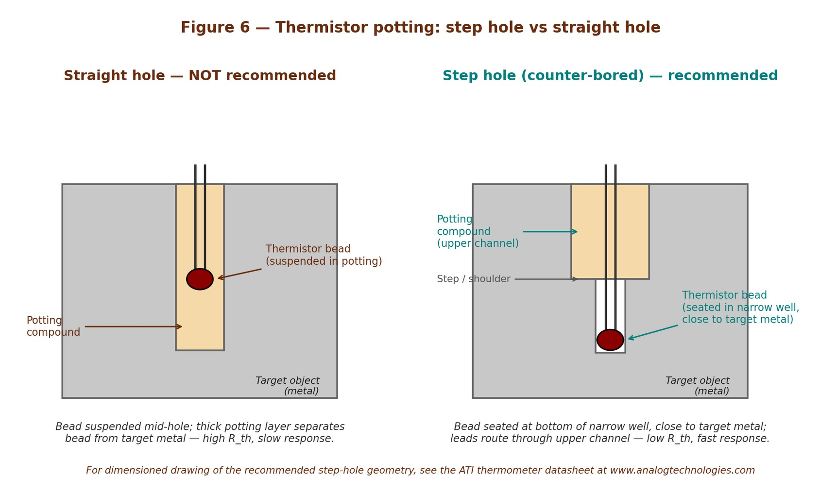
- Step-hole geometry for the sensor potting so the bead sits in close thermal contact with the target metal rather than mid-hole in potting compound.
Full mounting procedure (stack diagram, surface preparation, TIM selection and thickness, torque calculation from contact pressure, screw sequence, sealing and condensation management) is detailed in AWP-TECC-03, §10.
6. Temperature Sensor — Controller Compatibility
The temperature sensor closes the loop and sets the upper bound on resolution and response. The controller-side compatibility points are:
- NTC thermistor — the default sensor for ATI precision controllers (TEC14M, TECA1, TEC5V4A, TEC5V6A, high-current series), giving the highest sensitivity near 25 °C and the simplest voltage-divider readout.
- Platinum RTD (Pt100/Pt1000) — supported on selected ATI controllers where lowest long-term drift or widest temperature range is required, with the trade-off of lower sensitivity near 25 °C and the need for precision current excitation and lead-resistance compensation.
- Semiconductor IC sensors — used in the ATFC106D digital enclosure-cooling controller where ±1 °C precision is sufficient; not the recommended choice for precision continuous-current laser-diode or sub-10 mK applications.
ATI recommends pairing precision controllers with thermistors from the matched product line. Sensor placement (proximity to the load, step-hole vs straight-through-hole potting, sensor mounting thermal-resistance contribution to the stability budget, and the comparative selection table NTC vs RTD vs IC) is detailed in AWP-TECC-03, §8.
6b. Thermistor Linearization Network
An NTC thermistor’s resistance-versus-temperature curve is approximately exponential in 1/T (the β model). Reading the NTC with a simple two-resistor voltage divider produces an output voltage that is significantly nonlinear and that has a small voltage swing per °C — both of which complicate accurate closed-loop temperature regulation across a useful operating range. Setpoint scaling varies with operating point; loop gain becomes temperature-dependent in a way the compensation network must absorb.
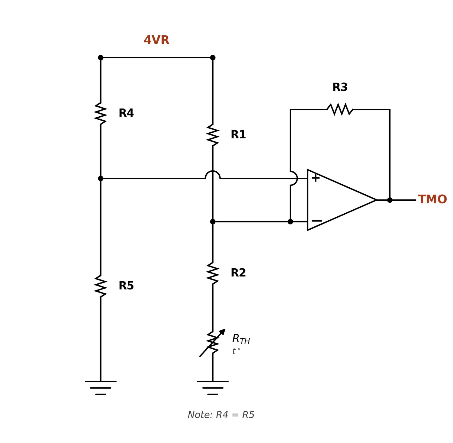
ATI precision controllers (TEC14M, TECA1, TEC5V4A, TEC5V6A) and the high-current series (TEC18V15A, TEC24V10A, TEC24V15A) include an on-module thermistor linearization network — a three-resistor network (R1, R2, R3) combined with an op-amp gain stage (R4, R5) — that produces a temperature-monitor output (V_TMO) that is engineered to be linear at three designer-chosen calibration temperatures and very close to linear in between. The result is a large, near-linear V_TMO swing across the calibrated temperature range, well suited to direct comparison against the setpoint (TMS) signal inside the closed loop.
Linearization equations
Given the NTC’s resistance at the three chosen calibration temperatures — R_LOW at T_LOW, R_MID at T_MID, and R_HIGH at T_HIGH (typically the middle of the operating range) — the three network resistors are calculated as:
R1 = R_MID + [ R_MID × (R_LOW + R_HIGH) − 2 × R_HIGH × R_LOW ] / [ R_HIGH + R_LOW − 2 × R_MID ]
R2 = R1 − R_MID
R3 = R1 × ( R1 + R_LOW − R_MID ) / ( R_LOW − R_MID )
R4 and R5 set the op-amp bias and gain and are typically equal (R4 = R5). The network is exact at the three calibration temperatures; the residual deviation between calibration points is small (typically tens of millivolts) for a 20 °C calibrated range using a typical 10 kΩ NTC.
Worked example — 10 kΩ NTC linearized across 15 / 25 / 35 °C
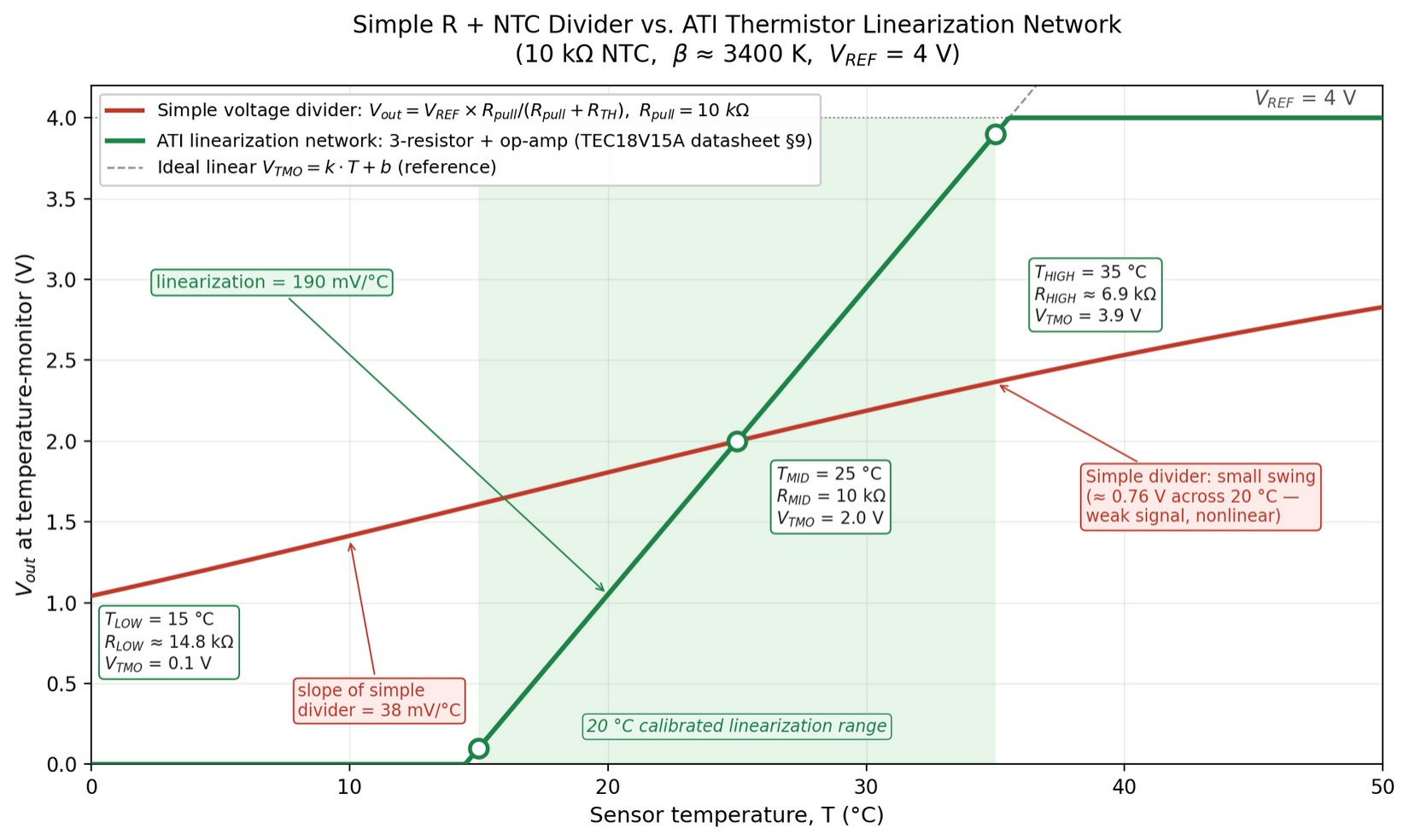
Taking the example from the TEC18V15A datasheet — a 10 kΩ NTC linearized over the 15–35 °C range that covers typical photonic and precision-instrument operating points:
| Quantity | Value | Reading |
|---|---|---|
| R_LOW at T_LOW = 15 °C | ≈ 14.8 kΩ | NTC resistance at the low calibration temperature |
| R_MID at T_MID = 25 °C | 10 kΩ | NTC resistance at the middle calibration temperature |
| R_HIGH at T_HIGH = 35 °C | ≈ 6.9 kΩ | NTC resistance at the high calibration temperature |
| R1 (computed) | 17.5 kΩ | Series bias resistor from V_REF to the network |
| R2 (computed) | 7.5 kΩ | Parallel linearization resistor |
| R3 (computed) | 81.3 kΩ | Op-amp feedback resistor (gain setting) |
With these values, V_TMO sweeps from ≈ 0.1 V at 15 °C, through ≈ 2.0 V at 25 °C, to ≈ 3.9 V at 35 °C — a ~3.8 V swing across the 20 °C range, equivalent to about 190 mV/°C. By comparison, a simple 10 kΩ pull-up divider with the same NTC produces only about 0.76 V swing across the same 20 °C range (about 38 mV/°C, a roughly 5× weaker signal per °C), and is visibly nonlinear.
Why this matters for closed-loop temperature regulation
- Larger signal swing per °C (~5× the simple-divider slope in the example above) gives the closed loop a stronger error signal, improving the loop’s effective resolution against the same ADC and noise floor.
- Linear V_TMO ↔ T mapping simplifies the relationship between setpoint voltage (TMS pin) and target temperature — engineers can scale setpoint directly in millivolts-per-millikelvin without a lookup table or per-unit calibration of the NTC curve shape across the operating range.
- Constant loop gain across the calibrated range — because dV_TMO/dT is approximately constant, the small-signal loop gain does not vary significantly with operating temperature, and a single compensation-network design holds across the full setpoint range without retuning at each operating point.
- Built into the controller — engineers do not need to design the linearization network externally. The three resistors and the op-amp gain stage are part of the standard ATI precision-controller architecture.
Pulse-mode vs. continuous-mode NTC excitation
The TEC18V15A and related precision controllers expose two NTC readout modes that trade off self-heating against simplicity:
- Pulse mode — R1 is connected to the pulsed reference (4VRS). The NTC is energized only briefly during each sample cycle, reducing average self-heating by approximately 10× compared to continuous excitation. Recommended when NTC self-heating would otherwise be a meaningful contributor to the stability budget — typical for small-bead NTCs, low-thermal-mass sensors, and stability targets below ~10 mK at the sensor. The SBDN pin should be in the 3.1–4.0 V range.
- Continuous mode — R1 is connected to the continuous reference (4VR). Simpler readout, slightly higher NTC self-heating. The SBDN pin should be in the 2.4–2.6 V range. Suitable for most general OEM applications where NTC self-heating is acceptable in the stability budget.
What the linearization network does — and does not — fix
Fixes
- The V_TMO-versus-T curve shape.
- The small voltage swing per °C of the raw divider.
- The temperature-dependent loop gain of the raw divider — across the chosen [T_LOW, T_HIGH] range.
Does not fix
- The NTC’s absolute resistance tolerance at room temperature (typically 1% or 2% per the chosen NTC grade).
- β-value tolerance, which translates into a slope error of V_TMO/T.
- NTC aging drift over service life (typically 0.02–0.1 °C/year depending on quality and operating temperature).
- NTC self-heating (which pulse mode reduces but does not eliminate).
- Sensor placement and mounting thermal resistance to the controlled object.
Part IV — ATI Product Guide
The five family groups, what each is for, and five worked examples that run the methodology end to end.
7. ATI TEC Controller Product Family Taxonomy
ATI manufactures TEC controllers organized into five family groups. The grouping is by architecture and supply voltage; within each group, current rating and precision grade differentiate specific part numbers.
| Family group | Members and roles | Architecture |
|---|---|---|
| TEC14M | TEC14M5V3R5AS — micro-form-factor SMT (14 × 14 × 2.2 mm), 5 V input, 3.5 A. | Hybrid |
| TECA1 | TECA1-3V-3V (3.3 V input) and TECA1-5V-5V (5 V input), each in -D / -DA / -DAH grades. General-purpose DIP, 2.5 A. | Hybrid |
| TEC5V | TEC5V4A (4 A) and TEC5V6A (6 A), each in -D / -DA / -DAH grades, with -NT and -LD variants. Mid-power workhorse, 5 V input, DIP. | Hybrid |
| High-current series (TEC18V15A, TEC24V10A, TEC24V15A) |
TEC18V15A: 6–18 V input, ±15 V output to TEC, up to 15 A. TEC24V10A: 5.5–25 V input (24 V nominal), up to 10 A. TEC24V15A: 5.5–24 V input, up to 15 A. The three controllers share footprint and pinout and are evaluated on a single shared eval board (TEC24V15AEV2.2). Built on ATI’s hybrid output stage, with added firmware-managed digital configuration — Auto-PID, programmable protections, digitally-set PID parameters, and digitally-set current and voltage limits. | Hybrid (with firmware-managed digital configuration) |
| ATFC | ATFC106D (12 V input, up to 12 V output to TEC). Digital window-mode controller with integrated heat-sink fan PWM, suited to enclosure cooling — the TEC is driven on when the load exceeds the upper window threshold and off when it falls below the lower threshold, rather than running continuous closed-loop bidirectional drive. | Digital window-mode enclosure-cooling controller; integrated fan PWM (not continuous-current precision drive) |
Naming standardization. The digital fan-controller product uses the ATFC prefix — Analog Technologies Fan Controller — with the trailing D indicating digital on/off output control. By contrast, the TEC prefix on the precision analog and high-current families indicates a closed-loop continuous-current TEC controller. The two prefixes signal architecturally different products.
29 years of product continuity for OEM TEC controllers
Across the company’s 1997–2026 history, applied to the TEC controller products currently in ATI’s catalog as of 2026, ATI’s operational record on transitions has been to communicate end-of-life in advance and offer an upgraded replacement intended to maintain functional compatibility — meaning the upgraded part is intended to be usable in the same application, though some level of qualification effort (and in some cases minor PCB or firmware adaptation) may be required depending on the specific transition. The exact migration path for any given part — pinout, footprint, electrical compatibility, and qualification effort — varies and is documented per-part. Request the migration details for the specific part you are designing in, and any formal long-term-supply statement required by your program, at sales@analogtechnologies.com. This operational record is one factor customers cite when staying with the line across multi-year product programs; it is not a contractual guarantee in this document.
TEC14M — when PCB space is the binding constraint
The TEC14M family is a 14 × 14 × 2.2 mm SMT module that delivers up to 3.5 A on a 5 V supply with the hybrid topology described in §3 — a compact module-level closed-loop TEC controller in the 3–4 A current class. In applications where PCB area is the binding constraint, the TEC14M is the ATI starting point.
For SMT TEC controllers at the upper end of their current rating, board-level thermal design matters: provide adequate copper pour beneath and around the module’s thermal-pad land, generous thermal vias to a continuous internal ground plane, and a clear air path so that conducted heat can spread away from the package. See the TEC14M datasheet for the recommended thermal-pad geometry, copper area, and via pattern, and confirm derating against the datasheet’s ambient-vs-current curve at the application’s worst-case ambient.
Ideal for: miniaturized OEM products, hand-held photonic sensors, dense optical-bench assemblies, fiber-laser butterfly packages where the controller must fit alongside the diode in a sealed module, wearable medical instruments.
TECA1 — general-purpose precision in DIP
The TECA1 xV-xV is the workhorse for prototyping and general OEM cooling at the 2.5 A class. The DIP package is breadboard-friendly and drops directly into a prototype PCB. Available in 3.3 V (-3V-3V) or 5 V (-5V-5V) input configurations, each in the three precision grades (-D, -DA, -DAH).
Ideal for: prototype evaluation, low-volume production, moderate-power laser-diode cooling, photodetector temperature control, OEM products at the 1–3 A operating-point range.
TEC5V4A / TEC5V6A — mid-power workhorse
The TEC5V series is widely used across ATI’s OEM customer base in 5 V production designs. Both members run on a 5 V supply and share the 25.4 × 19.9 × 8.8 mm DIP footprint. The TEC5V4A delivers up to 4 A; the TEC5V6A delivers up to 6 A. Available in D, DA, and DAH grades, with -NT and -LD variants.
Ideal for: higher-power laser-diode cooling (telecom DFBs, fiber-pump diodes, free-space optical sources), multi-stage TEC stacks where the operating point exceeds 2.5 A, mid-power photonics. TEC5V6A-DAH is the recommended starting point for any application requiring DAH-grade precision at 4–6 A.
TEC18V15A, TEC24V10A, TEC24V15A — the high-current series
The high-current series is ATI’s family for higher-power applications where the 5 V precision families cannot supply the required combination of voltage and current. The series has three members in active production that share footprint, pinout, and evaluation board (TEC24V15AEV2.2). The TEC18V15A accepts a 6–18 V input range and delivers ±15 V to the TEC at up to 15 A. The TEC24V10A accepts a 5.5–25 V input range (24 V nominal) and delivers up to 10 A, suited to the 24 V rail standard in industrial automation and telecom infrastructure. The TEC24V15A combines a wide 5.5–24 V input range with up to 15 A output, spanning 12 V and 24 V applications with a single part number.
- Auto-PID compensation. The compensation network is identified and tuned automatically when a new load is connected, removing the manual tuning step that is otherwise needed for non-standard thermal loads. The host system can re-trigger identification if the thermal load changes during the product’s lifecycle. Engineers must still validate the resulting tuning against the actual thermal load on an evaluation board before locking the design.
- Programmable protections. UVLO, OVLO, I-limit in the heating direction, I-limit in the cooling direction, V-limit in the heating direction, and V-limit in the cooling direction are individually programmable. Typical use is a tighter limit in the cooling direction (where Joule self-heating compounds the thermal load) than in the heating direction. The protections operate continuously without host intervention.
- Low conducted noise back into the power supply. The firmware-managed output stage is designed to limit the switching transients that propagate back into the V_PS supply rail, through a combination of soft-switching on the output FETs and on-board filtering between the switching stage and the V_PS input. See family datasheet for measured conducted-noise values.
- Zero-crossing current management. When the loop reverses direction, the output current crosses zero in a managed transition that avoids large discontinuities. This can help maintain smoother regulation near setpoint in applications that hover at the cooling-heating boundary; the magnitude of the improvement depends on the specific application thermal dynamics and the loop tuning.
- Firmware-managed loop tuning. Beyond the Auto-PID identification step, the firmware implements transient-response shaping intended to support faster ramp times in slewing applications such as PCR thermal cyclers, while preserving stability margin at steady state.
Ideal for: large TECs, multi-TEC arrays, deep-cooling applications (cooled imaging sensors, mid-IR detectors), industrial process cooling, medical instruments with slewing thermal profiles, applications requiring continuous electrical protection without host firmware intervention. Choose TEC18V15A for flexible 6–18 V supplies and maximum 15 A current; choose TEC24V10A for installations standardized on the 24 V rail at 10 A; choose TEC24V15A when the design needs maximum current capability across a wide input-voltage envelope.
ATFC106D — digital TEC + fan control
The ATFC family is architecturally distinct from the rest of the line. The ATFC106D is a digital on/off controller designed for enclosure-cooling applications where the TEC and the heat-sink fans must be coordinated automatically without host firmware. Window-mode setpoint operation (cooling when the load is above the upper window limit, holding when inside the window, optionally heating when below the lower limit) suits kiosks, refrigerated displays, and outdoor electronics enclosures.
The ATFC106D operates on a 12 V input at up to 20 A, delivers up to 12 V across the TEC, and includes integrated PWM control for two cooling fans, in a boxed module measuring approximately 152.6 × 76 × 20.4 mm. Bench evaluation against the actual thermal load is required before locking the production design.
The ATFC106D is intended for window-mode enclosure / appliance cooling and is not the recommended starting point for continuous bidirectional precision object-temperature regulation. Sub-10 mK and millikelvin-class object-temperature applications should use the precision-analog hybrid families (TECA1, TEC5V4A, TEC5V6A, TEC14M) or the high-current series, where the fan-PWM dynamics and on/off output transitions would otherwise compromise stability.
Ideal for: kiosks, vending machines, refrigerated displays, outdoor electronics cabinets, lab incubators, and any “appliance” product where the TEC controller operates invisibly without host firmware intervention.
Evaluation boards
ATI ships matched evaluation boards for the precision analog families. The compensation-network components are accessible for tuning iteration without rebuilding a PCB. TEC connectors, thermistor inputs, supply jacks, and diagnostic test points are populated and labeled.
| Evaluation board | Compatible controllers | What it provides |
|---|---|---|
| TEC14MEV1.0 | TEC14M5V3R5AS only | 140 × 130 mm carrier with the micro-form-factor TEC controller pre-installed; banana jacks for supply; TEC and thermistor harness; diagnostic test points. |
| TECEV104 | TECA1-xV-xV (D, DA, DAH); TEC5V4A and TEC5V6A (D, DA, DAH) | Complete tuning and application circuit; LED temperature-status indicator; multiple connection pads for external instruments; supports setpoint configuration and compensation-network tuning against the user’s actual thermal load. |
| TEC24V15AEV2.2 | TEC18V15A, TEC24V10A, TEC24V15A | Shared evaluation board for the entire high-current series. Supports Auto-PID identification against the user’s thermal load, programmable I/V limits, and compensation-network tuning. The three controllers share footprint and pinout; the same eval board is used to evaluate each one. |
| (no separate eval board required) | ATFC106D | The ATFC106D is its own evaluation fixture. Bench-test the unit against your actual thermal load, ambient envelope, and fan in your enclosure before locking the production design. |
Evaluate before designing in
ATI provides evaluation boards for each precision controller family to qualified OEM projects, supporting validation of compensation tuning, current and voltage limits, and protection thresholds against the actual TEC and thermal load before a custom PCB is committed. To request an evaluation board matched to your application, contact sales@analogtechnologies.com with your thermal load, supply rail, and target controller family.
8. Illustrative Application Examples
The five worked examples below illustrate the six-step methodology end-to-end. Each starts with the application’s requirements, walks through the selection inputs, and arrives at a specific recommended controller. These examples are illustrative — exact part-number recommendations for a specific project should be confirmed with ATI applications support against the actual thermal load and operating envelope.
Regulated-application notice. ATI TEC controllers, TEC modules, and thermistors are commercial-grade components. The examples below illustrate the engineering selection methodology and are starting points for engineering evaluation. Component selection in this guide does not constitute medical, automotive, aerospace, or other regulatory qualification of the end product. The OEM is responsible for validating the complete system under its actual electrical, thermal, mechanical, environmental, safety, and regulatory requirements, including any required certifications.
Example 1 — Laser-diode wavelength stabilization
A telecom DFB laser diode in a butterfly package must be held to a wavelength stability of approximately 0.1 pm to meet the channel-grid requirement of a dense WDM system. The wavelength temperature coefficient of the diode is approximately 0.08 nm/°C, so 0.1 pm wavelength stability requires roughly ±0.0012 °C temperature stability at the diode junction. The host transponder card provides a 5 V supply rail; PCB area is moderately constrained but not extreme.
Working through the methodology: the cold-side thermal load is in the 1–3 W range (diode dissipation plus parasitics through the lead frame). Worst-case ambient at the heat sink is around 70 °C inside the transponder enclosure, giving a required ΔT of approximately 45 °C from the 25 °C diode setpoint. A single-stage TEC sized to operate at 60–70% of its I_max at this ΔT typically draws 1.5–2 A. The controller’s I_max must comfortably exceed this; both the TECA1 (2.5 A) and the TEC5V4A (4 A) are in range. The DAH precision grade is required to support the millikelvin stability target.
Recommended controller: TECA1-5V-5V-DAH for the lower-end thermal-load case (1–2 W), or TEC5V4A-DAH for the higher-end case (2–3 W) where extra current headroom helps with cool-down transients. The 5 V supply matches typical transponder rails; the hybrid topology helps reduce switching-ripple and EMI risk to the wavelength-locker electronics, subject to layout, grounding, cabling, and filtering. The -LD variant of the TEC5V family is pre-configured for laser-diode thermal time constants and typically reduces the manual compensation-tuning effort for common DFB, VCSEL, and Fabry-Pérot packages.
Illustrative calculation. The wavelength-stability and temperature-stability numbers used in laser-diode examples in this guide are illustrative engineering calculations, not guaranteed product-level performance. Achievable wavelength stability at the diode junction depends on the specific diode’s dλ/dT coefficient (which varies by manufacturer, wavelength, drive current, and aging), package thermal coupling between the TEC and the diode chip, sensor placement and self-heating, current-driver stability, optical feedback, ambient stability, and the full system architecture. Controller stability is measured at the sensor under defined laboratory conditions; junction-level stability requires the full thermal stack to be designed and validated.
Example 2 — Medical diagnostic instrument: PCR thermal cycler
A single-well PCR thermal cycler must slew between 4 °C (annealing) and 95 °C (denaturation) at ramp rates of 3–5 °C per second, with stability of approximately ±0.1 °C at each plateau. The thermal load is dominated by the aluminum well block and reagent mass, totaling 10–30 W during the ramp phase and dropping at the hold. The application requires bidirectional drive and high current to deliver the slew rate the chemistry demands.
Working through the methodology: the worst-case ΔT (heat-sink hot side around 60 °C, cold side at 4 °C) is approximately 56 °C, well within Bi₂Te₃ single-stage range. The TEC operating point at 60–70% of I_max under these conditions typically draws 8–12 A at 12–15 V. Neither the 5 V families nor the ATFC enclosure-cooling family fits this combination of voltage and current. The slew-rate requirement also favors a family with firmware-managed control.
Recommended controller: TEC18V15A. The 6–18 V input matches typical medical-instrument supplies; the 15 A capability delivers headroom for the ramp; the ±15 V output drives the deep-ΔT operating point; the Auto-PID feature handles the unit-to-unit variation in well-block thermal mass common across production builds; the low conducted noise back into the V_PS supply rail is an important consideration when the same supply feeds the instrument’s optical readout electronics.
Example 3 — Outdoor kiosk display cooling
An outdoor digital signage display includes a sealed electronics compartment that must be held below 40 °C internal temperature across an ambient range from −10 °C (winter night) to +55 °C (sunlit cabinet on a hot day). The compartment thermal load — cabinet leakage plus display driver electronics — runs 30–60 W depending on operating mode. The application requires autonomous operation with no host firmware involvement and integrated control of the heat-sink fans.
Working through the methodology: the application is fundamentally enclosure cooling rather than precision temperature regulation. The setpoint is a window — “keep below 40 °C” — not a point. The fan must be coordinated with the TEC drive. The supply rail is typically 12 V in signage installations. The high-current group is over-specified; the precision families are over-engineered for the ±2 °C window-mode tolerance the application allows.
Recommended controller: ATFC106D. Window-mode setpoint matches the application directly. Integrated fan PWM handles airflow without external circuitry. 12 V supply matches the signage power rail. Plug-and-play deployment reduces firmware development effort, though bench evaluation against the deployed thermal load and ambient envelope is still recommended before fielding the product.
Example 4 — Miniaturized photonic sensor module
A hand-held Raman spectrometer integrates a cooled InGaAs photodetector for the 900–1700 nm response band. The detector requires 30 °C below ambient to suppress dark current to the design level. The thermal load is small (0.5 W) but the form-factor constraint is severe — the controller must fit on a 30 × 30 mm carrier alongside the detector, its bias circuitry, and the trans-impedance amplifier. The hand-held form factor also dictates a 5 V battery-derived supply.
Working through the methodology: the thermal load is well within the smallest available family (TEC14M, 3.5 A). The form-factor constraint excludes the DIP packages of the TECA1 and TEC5V families. The hybrid topology is important for keeping switching noise out of the trans-impedance amplifier’s input; a pure-PWM controller would couple ripple into the detector’s bias rail and corrupt the dark-current spectrum. Stability of ±0.05 °C is more than adequate.
Recommended controller: TEC14M5V3R5AS. The 14 × 14 mm SMT footprint is the only family that fits the carrier; the 3.5 A rating gives substantial headroom over the 0.5 W load; the hybrid topology delivers the low ripple needed alongside a sensitive detector front end. The matched TEC14MEV1.0 eval board is the recommended starting point for compensation tuning against the actual carrier.
Example 5 — LIDAR receiver cooling
A long-range LIDAR receiver uses a cooled avalanche photodiode (APD) to detect the 905 nm return pulses. The APD’s dark current and gain stability are strong functions of temperature, requiring stability of approximately ±0.01 °C to hold the detection threshold within calibration. The thermal load is 3–5 W. The detector sits in front of a low-noise trans-impedance amplifier whose noise floor must not be compromised by controller-radiated EMI. The supply is a 5 V derived rail.
Working through the methodology: the thermal load and ΔT point to the TEC5V family. The stability target (±0.01 °C) points to the DAH precision grade. The noise environment — TIA in the controller’s electrical neighborhood — strongly favors the hybrid topology over pure-PWM. The pulsed nature of LIDAR operation creates transient thermal loads during high-rep-rate measurements; current headroom matters.
Recommended controller: TEC5V6A-DAH. The 6 A capability gives comfortable margin over the steady-state thermal load and absorbs the bursty transient loads during pulse operation. The hybrid topology delivers the low ripple required for noise-sensitive front-end electronics. The DAH grade provides the setpoint precision needed for tight dark-current control. The 5 V rail matches typical APD-receiver supplies.
Part V — Decision Support
Answers to the questions that come up most often, and the inputs ATI applications engineering needs to make a recommendation.
9. Frequently Asked Questions
How do I design a TEC cooling system?
Five components must be selected and sized together against the application’s thermal load, ambient envelope, and target setpoint: (1) the TEC module, (2) the heat sink on the hot side, (3) the TEC controller, (4) the temperature sensor on the load, and (5) the mechanical mounting between the load and the heat sink. The standard sequence is: characterize the cold-side thermal load Q_load (active plus passive); specify the worst-case ambient at the heat sink; size the heat sink by R_hs ≤ (T_hot,max − T_ambient,max) ÷ Q_hot; select a TEC module that delivers the required Q_load at the resulting ΔT; match a TEC controller with 1.5–2× current and voltage margin to the TEC’s operating point; place a small NTC thermistor on the cold plate within 5 mm of the load; and mount the TEC with thin uniform TIM on both ceramic faces, label / cold side toward the load, under uniform compression. Validate the integrated stack on an evaluation board against the actual load before locking the design.
How do I choose a TEC controller?
Work through six steps: (1) calculate the cold-side thermal load Q_load, (2) define target setpoint and worst-case ambient, (3) select a TEC and read its operating-point current and voltage from the datasheet, (4) match a controller whose I_max and V_max exceed those values with 1.5× to 2× margin, (4b) confirm the controller’s input voltage matches your system supply rail, (5) choose the design priority that determines family (size, power, ΔT, or autonomous enclosure cooling), and (6) size the heat sink for Q_hot = Q_c + P_electrical with appropriate margin. Section §4 covers the full methodology.
What is the difference between a TEC controller and a TEC driver?
A TEC controller closes the temperature control loop itself — it reads a sensor, compares to a setpoint, and adjusts TEC current automatically to maintain the load at the target temperature. A TEC driver is open-loop: it delivers a commanded current without temperature feedback, leaving the host system to close the loop in firmware. Controllers are appropriate when temperature stability is the deliverable; drivers are used when the host already implements thermal logic.
Can I drive my TEC with PWM directly, without a controller?
Direct unfiltered PWM into a TEC is generally a poor choice for precision temperature control: the ripple current produces I²R Joule heating that competes with Peltier cooling, and the switching edges radiate EMI. Direct PWM can be acceptable for non-precision, non-EMI-critical low-cost cooling, where its simplicity and low component count are advantages. For OEM products with stability or low-noise specifications, the LC-filtered output of a proper controller — or, better, the hybrid topology — can reduce the efficiency penalty associated with ripple-induced Joule heating and substantially reduces both conducted and radiated EMI. System-level EMC validation still requires standard layout, grounding, shielding, and filter design at the integration level.
How do I know if my TEC controller has enough current?
Two sizing strategies are recommended as starting points. Strategy 1, the practical OEM approach: determine the TEC’s operating-point current at approximately 60–70% of the TEC’s I_max from the TEC datasheet at the worst-case ΔT — a reasonable starting balance between TEC size, COP, and reliability. Strategy 2, the high-COP / long-life approach: operate the TEC at 25–30% of its I_max with an oversized TEC, for battery-powered or long-life applications where efficiency outweighs minimum TEC size. In both strategies, the controller’s rated I_max must exceed the chosen operating-point current with a 1.5× to 2× safety margin to handle cool-down transients and worst-case ambient excursions; controller V_max must exceed the operating-point V_TEC with headroom for dropout, supply tolerance, and wiring drop. These are starting heuristics — final sizing should be verified against the specific TEC datasheet curves and lab measurements on the actual load.
What about inrush current at power-on?
ATI controllers limit output current to their programmed I-limit setting from power-on; they do not deliver a step current to a cold TEC. For the high-current series (TEC18V15A, TEC24V10A, TEC24V15A), the firmware ramps the loop output gradually as it identifies the load via Auto-PID, minimizing transient draw from the V_PS rail. Engineers concerned about upstream supply protection can set the I-limit lower than the controller’s rated I_max to establish a fixed inrush ceiling that matches the upstream fuse or current-limited supply.
What happens if I exceed the TEC’s maximum current?
Three consequences, in increasing severity. COP drops below 1, so every watt of electrical power produces more than a watt of heat at the hot side — defeating the purpose of cooling. TEC pellets experience thermal-mechanical stress that accelerates fatigue and shortens module life. In extreme cases, the solder joints inside the TEC melt or migrate, causing permanent damage. Controllers with proper current-limit protection prevent this — ATI controller families include current-limit protection; see the relevant family datasheet for the specific implementation and adjustability options.
Can one TEC controller drive multiple TECs?
Yes, within the controller’s combined voltage and current budget. Multiple TECs can be wired in series (voltage adds, current stays the same — total V across the string must stay below controller V_max), in parallel (current adds, voltage stays the same — sum of TEC currents must stay below controller I_max), or in hybrid series-parallel configurations. Module ratings must match — mismatched modules in parallel will current-share unequally and the weaker ones fail first. For arrays larger than 2–3 modules, the high-current series is generally appropriate; detailed array design must follow the controller’s combined power rating and TEC matching rules.
Do I need a heat sink on the TEC controller itself?
Depends on family and operating point. Pure-linear architectures (not used in ATI’s current catalog) dissipate V_drop × I_out in the linear pass element and require substantial controller-side heat sinking; ATI’s hybrid topology dissipates substantially less because the bulk current is delivered by the switching leg and only a small fraction of the headroom is dropped across the linear post-regulator. In practice, the precision-analog hybrid families typically need no dedicated controller heat sink in normal operation. The high-current series — also hybrid, at higher absolute current — may benefit from a chassis-mount thermal interface at sustained worst-case load; the product datasheet specifies the thermal derating curve.
What is the difference between the -D, -DA, and -DAH variants?
Setpoint voltage accuracy. The -D variant guarantees ≤5 mV setpoint error (approximately 0.05 °C with a standard 10 kΩ NTC). The -DA variant tightens this to ≤2 mV (approximately 0.02 °C). The -DAH variant tightens further to ≤0.5 mV (approximately 0.005 °C). The closed-loop stability around the setpoint mean is typically much tighter than the setpoint accuracy itself — see §5. Specify the lowest grade that meets the stability requirement; higher grades cost more without performance benefit if the application does not need them.
How do I set the temperature setpoint?
Three options. Apply an external DC voltage to the setpoint input pin — typically set by a DAC, an external precision reference, or a potentiometer. Use an external resistor divider from an internal reference, for fixed-temperature applications. Use the digital interface on the ATFC106D for software-controlled setpoint adjustment. The temperature range network (§5b) maps the setpoint voltage to actual temperature; standard variants use a fixed range, -NT variants allow custom range configuration.
Can I use a TEC controller for heating only?
Yes. The same controller drives the TEC in either polarity automatically — if the load is below setpoint, the controller heats; if above, the controller cools. For heating-only applications, the bidirectional capability is unused but not harmful. In an idealized heat-pump model, heating mode COP is greater than cooling mode COP because Joule dissipation adds to the Peltier heat delivered; the practical advantage depends on the operating point and system losses.
What is the typical lifespan of a TEC controller?
ATI controllers are designed for continuous operation supporting the long service lives required by OEM industrial and medical products. Capacitor aging is the dominant wear-out mechanism in switch-mode designs; the linear stages of the hybrid topology have no electrolytic capacitors in the signal path. For specific MTBF figures applicable to a particular family and operating profile, request the relevant reliability statement from ATI.
10. Summary and Selection Support
Selecting a TEC controller is a structured decision, not a guess. The six-step methodology in this paper takes the engineer from a thermal-load requirement to a starting ATI part number, with the trade-offs laid out at each step; final selection is confirmed against the actual load and constraints before locking the design.
Six-step checklist
- Define cold-side thermal load Q_load — sum of device dissipation, conduction, convection, and radiation. Add 30–50% for parasitics if estimating.
- Define target temperature and ambient range — setpoint, worst-case ambient at the heat sink, required ΔT across the TEC.
- Select the TEC module — choose the 60–70% practical sizing strategy for general OEM cooling, or the 25–30% high-COP strategy for battery-powered or long-life applications. Read I_tec and V_tec from the TEC datasheet at the operating point.
- Match controller to TEC — controller I_max ≥ 1.5× I_tec, V_max ≥ V_tec, supply voltage compatible with system. See Step 4b for input-voltage selection.
- Choose design priority — power, size, ΔT, or autonomous enclosure cooling — and map to ATI family.
- Size the heat sink — for Q_hot = Q_c + P_electrical at worst-case ambient. R_hs ≤ (T_hot,max − T_ambient,max) / Q_hot with margin appropriate to the operating environment.
Selection-support form
Engineers who prefer a recommendation to a calculation can send ATI applications engineering the following information. Applications engineering review is available for qualified OEM projects.
| Application | Brief description (laser cooling, medical instrument, photonic sensor, enclosure cooling, etc.) |
| Cold-side thermal load Q_load | Watts at worst case |
| Target temperature setpoint | Fixed value or range |
| Worst-case ambient at heat sink | °C |
| Available supply rail | 5 V, 12 V, 24 V, etc. |
| Required stability | Peak-to-peak over operating window |
| EMI / noise environment | Critical analog circuits nearby? (laser driver, TIA, precision ADC) |
| Size / package preference | SMT vs. DIP vs. boxed module; PCB area constraint |
| TEC part number (if known) | Or attach datasheet |
| Heat-sink configuration (if known) | Passive, forced-air, or liquid |
Quick decision matrix
First fork — what kind of temperature control? ATI’s TEC controllers split into two architectural categories. Use the precision continuous-current families for object-temperature control where the load must hold a setpoint (laser diodes, photodetectors, imaging sensors, PCR blocks, biosensors). Use the ATFC digital window-mode controller for enclosure-cooling applications where the load only needs to stay within a comfort window (kiosks, outdoor cabinets, refrigerated displays).
- Precision object-temperature control → TEC14M / TECA1 / TEC5V4A / TEC5V6A / TEC18V15A / TEC24V10A / TEC24V15A
- Enclosure cooling with fan / window-mode control → ATFC106D
Second fork — within precision, what design priority? The matrix below maps load range and design priority to a starting family and example part number.
| If you need… | Load range | Family group | Example part number |
|---|---|---|---|
| Smallest possible footprint | ≤ 1 W | TEC14M (14 × 14 mm SMT) | TEC14M5V3R5AS |
| General OEM prototyping | 1–3 W | TECA1 (DIP) | TECA1-5V-5V-DAH |
| Lower-mid-power 5 V design | 2–4 W | TEC5V (hybrid topology, 4 A) | TEC5V4A-DAH (or -LD for laser diodes) |
| Mid-power 5 V design | 4–10 W | TEC5V (hybrid topology, 6 A) | TEC5V6A-DAH (or -LD for laser diodes) |
| High current / high ΔT | 10–50 W | High-current series | TEC18V15A (6–18 V), TEC24V10A (24 V), or TEC24V15A (5.5–24 V flexible) |
| Autonomous enclosure cooling | 20–60 W | ATFC (window mode + fan PWM) | ATFC106D (12 V) |
Why ATI for OEM TEC controllers
The hybrid topology in ATI’s precision controller line (U.S. Patent 6,486,643 B2) delivers high efficiency together with low output ripple in the same module — combining the efficiency advantage of switching designs with the low-ripple advantage of linear designs by routing the bulk current through a switching leg and post-regulating the residual through a linear leg — substantially reducing the external LC filtering that pure-PWM controllers typically require for precision TEC drive, while avoiding the controller-cooling penalty of pure-linear designs. System-level EMC validation (layout, grounding, shielding) is still the engineer’s responsibility.
Practical reasons OEM engineers and procurement select ATI:
- One supplier for the matched controller, TEC module, and precision thermistor — fewer vendor relationships, faster bench bring-up, simpler BOM management.
- ATI’s matched thermistors are characterized with the tolerance and beta used in the precision controllers’ setpoint calculation, which simplifies calibration and supports DAH-grade setpoint precision when used with the specified ATI thermistor family, the intended R1/R2/R3 linearization network values, and the datasheet mounting and readout conditions. Final achievable precision depends on sensor placement, mounting, and system-level thermal design.
- Evaluation boards for every precision family, with the high-current series sharing the TEC24V15AEV2.2 platform — lower up-front evaluation cost and faster decision-to-prototype cycle.
- US-based applications engineering reachable by email and phone, with design review and starting-family recommendations for qualified OEM project specifications.
- 29-year track record of providing migration paths when products transition, which reduces requalification risk on multi-year OEM programs in regulated markets.
- Custom engineering for special and high-volume applications — customized TEC modules, customized TEC controllers, and complete custom TEC assemblies and systems.
Note for medical, automotive, aerospace, and other regulated applications. ATI TEC controllers, TEC modules, and thermistors are commercial-grade components intended as building blocks. When integrated into medical devices, automotive systems, aerospace equipment, or other regulated end products, system-level qualification, traceability, change control, and regulatory submissions (FDA, IEC 60601, ISO 13485, AEC-Q, RTCA DO-160, etc.) are the system designer’s responsibility. ATI does not represent that any standard catalog product is qualified for a specific regulated end use; contact ATI sales early in the design cycle to discuss documentation, lifecycle commitments, and any custom requirements your program needs.
Custom engineering for special and high-volume applications
Beyond the standard catalog, ATI takes on TEC-related engineering projects for OEM customers whose requirements fall outside the standard product line. This covers three project types:
- Customized TEC modules. Non-standard form factors, footprints, electrical ratings (I_max, V_max, Q_c), ΔT ranges, top-plate and bottom-plate materials, multi-stage configurations, and long-life construction matched to specific service-life and thermal-cycling profiles.
- Customized TEC controllers. Non-standard supply rails, footprint and pinout adaptations, suffix and variant combinations outside the standard offering, OEM-specific firmware configuration on the high-current series, and integration features such as host-side telemetry, fault reporting, and remote-setpoint interfaces.
- Custom TEC assemblies and systems. Complete delivered subassemblies — matched controller + TEC module + heat sink + temperature sensor, integrated and tested by ATI as a single deliverable.
Custom engineering work is appropriate for OEM volume programs and for special applications where the standard catalog does not match the requirement exactly. Engage early in the design cycle — typically before PCB layout is locked — so ATI engineering can scope the project, propose a path that minimizes non-recurring engineering cost, and define the prototype-to-production transition.
Next step — order the matched evaluation board for your application
The fastest path from this guide to a working prototype is to order the eval board that matches your design priority and validate compensation tuning against your actual thermal load before committing to a PCB layout. By application: miniature SMT and ≤ 1 W cold-side load → TEC14M5V3R5AS with the TEC14MEV1.0 board; 5 V laser-diode or photonic cooling at 1–3 W → TECA1-5V-5V-DAH with the TECEV104 board; mid-power 5 V precision OEM cooling at 4–10 W → TEC5V6A-DAH with the TECEV104 board (or the -LD variant for laser-diode loads); high-current applications at 10–50 W → TEC18V15A, TEC24V10A, or TEC24V15A — all three are evaluated on the shared TEC24V15AEV2.2 board; autonomous enclosure cooling at 20–60 W → ATFC106D, which serves as its own evaluation fixture.
Regulated-Use and Application-Safety Caveats
The application examples, product recommendations, and methodologies in this guide are engineering starting points for design evaluation, not certified design solutions. The OEM is responsible for validating the final product against all applicable electrical, thermal, mechanical, environmental, safety, regulatory, and end-application requirements before production.
Medical, diagnostic, and IVD applications: design and qualification must meet the relevant regulatory framework (e.g., FDA, IEC 60601, IEC 61010, IVDR / IVDD) — TEC sub-system performance is one input to that qualification, not a substitute for it.
Automotive and safety-related LIDAR systems: require system-level qualification, functional-safety analysis (e.g., ISO 26262), environmental testing, EMC compliance, and any applicable AEC-Q component qualification before deployment.
AI / GPU / large-area high-heat-flux electronics: TEC cooling is appropriate for localized hotspots, optical receivers, detector chips, reference sources, or other small-area thermal control unless a full system thermal design and validation prove otherwise — TEC technology is not a general substitute for liquid or two-phase cooling at large GPU package-level heat loads.
Sub-millikelvin and sub-10 mK applications: quoted stability figures are at the sensor under defined laboratory conditions; achievable stability at the controlled object depends on the full thermal stack and must be validated on the assembled system.
References
- G. Liu, “Thermoelectric Cooler Controller,” U.S. Patent 6,486,643 B2, issued Nov 26, 2002. Assigned to Analog Technologies, Inc.
- Analog Technologies, Inc., AWP-TECC-01, What Is a TEC Controller? — A Visual Engineering Guide. Rev. 4.0, 2026.
- Analog Technologies, Inc., AWP-TECC-03, How to Design a TEC Cooling System. 2026.
- Analog Technologies, Inc., AWP-TECM-01, What Is a Thermoelectric Cooler? 2026.
- Analog Technologies, Inc., AWP-TECM-03, Multi-TEC Thermal System Design. 2026.
- Analog Technologies, Inc., AWP-HS-01, How to Design a Heat Sink for a TEC Controller System. Forthcoming, 2026.
- D. M. Rowe, ed., Thermoelectrics Handbook: Macro to Nano, CRC Press, 2006.
- IEC 60751:2008, Industrial platinum resistance thermometers and platinum temperature sensors.